Expected Value Explained: Formula and Practical Examples

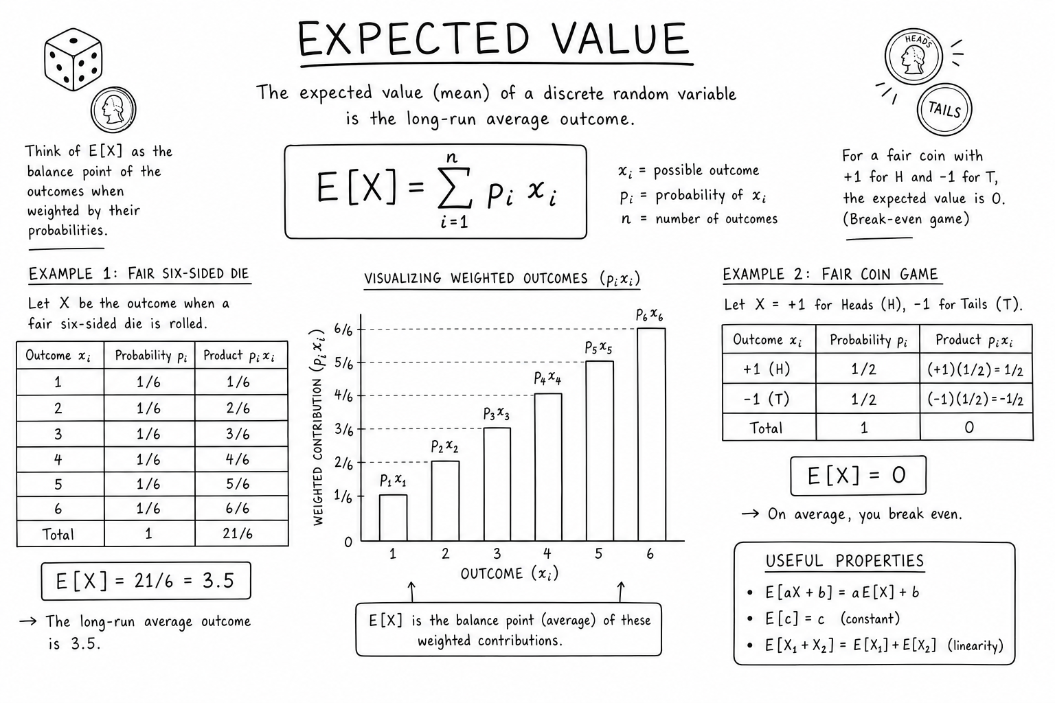
Expected value is a probability-weighted average: multiply each possible outcome by its probability, then add the results. You can use it to compare uncertain choices while keeping the assumptions visible.

For example, a $15,000 project with a 30% chance of closing has expected revenue of $4,500. A $5,000 project with a 90% chance also has expected revenue of $4,500. Assuming a rejected proposal earns nothing, the two tie before costs.

I wouldn’t choose between them on that number alone. Proposal time, delivery costs, payment timing and the consequences of earning nothing could change my choice.

What Is Expected Value?

Expected value weights each possible outcome by how likely it is. For repeated decisions under the same model, it describes the long-run average per attempt. You can also calculate it for a one-time decision; it still won’t tell you which outcome will happen.

For outcomes x_i with corresponding probabilities p_i, the expected value formula is:

$$E[X] = \sum_{i=1}^{n} p_i \, x_i = p_1 x_1 + p_2 x_2 + \dots + p_n x_n$$

The probabilities must add up to 1, or 100%. The outcomes can be money, hours, units sold, customers kept, anything you can put a number on.

The simplest bet shows how it works. A coin flip pays you $100 on heads and costs you $50 on tails.

$$E = (0.5 \times \$100) + (0.5 \times -\$50) = \$50 – \$25 = \$25$$

The expected value is $25 per flip. That number deserves a second look, because no single flip ever pays $25. Each flip pays $100 or takes $50, and $25 is what the two results average out to once they’re weighted by their chances. Expected value is an average, and it is not necessarily the most likely result or even a result that can occur in one attempt.

I’d check whether the possible $50 loss is affordable before considering the coin game’s positive expected value. A lower expected value can be a rational choice when the downside would hurt you more than the matching gain would help.

How to Calculate Expected Value

The arithmetic is multiplication and addition. I would spend more time checking the scenarios, costs and probabilities before calculating the total:

1. Define the decision and the period. Name the choice you’re pricing and the window it covers, whether that is one year, 3 years or the life of the project.
2. List the scenarios. Write down every way this could turn out, from a big win to a serious loss.
3. Put a net outcome on each scenario. Net means after the costs that belong to that scenario.
4. Estimate the probabilities. Use what you have: your own history with similar decisions, industry base rates or an honest expert judgment.

Then multiply each outcome by its probability and add the results. Say you’re pricing a product launch, and the net results over the launch period look like this:

Outcome	Probability	Net outcome	Contribution to expected value
Massive success	10%	$500,000	$50,000
Solid success	25%	$200,000	$50,000
Modest success	30%	$50,000	$15,000
Break-even	15%	$0	$0
Minor loss	15%	-$75,000	-$11,250
Major failure	5%	-$300,000	-$15,000
Total	100%		$88,750

The launch has an expected net value of $88,750 under these assumptions. It also has a 20% chance of a loss and a worst listed outcome of losing $300,000. I’d keep all three figures together when considering the decision.

Before trusting any table like this, run a short setup check:

• the scenarios don’t overlap and nothing likely is missing, so the probabilities account for the whole model
• every outcome uses the same units and the same period
• the probability column adds up to exactly 100%

How to Use Expected Value to Compare Options

I’d compare the expected value with the realistic alternative, including doing nothing or using the same resources elsewhere.

For the launch above, doing nothing is worth $0, so the $88,750 is the whole premium for taking the risk. If the same budget could earn a near-certain $50,000 elsewhere, the launch is worth $38,750 more in expectation than the safe route, and that $38,750 is what you’re being paid to accept a 20% chance of a loss. Whether that is a fair trade depends on how the loss would land on you, and the arithmetic can’t answer that part.

The same scale also works across options that look nothing alike. Say you have $10,000 for marketing and 3 ways to spend it:

Option	Chance it works	Revenue if it works	Revenue if it doesn’t	Expected revenue	After the $10,000 cost
Facebook ads	50%	$35,000	$5,000	$20,000	$10,000
Influencer campaign	25%	$100,000	$2,000	$26,500	$16,500
Trade show	90%	$20,000	$12,000	$19,200	$9,200

These figures are expected revenue less campaign cost; they exclude product and delivery costs. The influencer example has the highest value on that limited measure, but its failure outcome returns only $2,000 against $10,000 spent. The trade-show example has a lower expected result and less variation between its two outcomes. I’d include the remaining costs and decide what downside is affordable before choosing.

How Likely Does Success Need to Be?

This is the question I’d add to every expected value calculation, because it turns a guessed probability into a threshold you can test. Instead of defending one estimate, work out the probability at which the decision breaks even, then ask whether your evidence clears it.

Take a software feature. Building it costs $80,000. If it succeeds and brings in new customers, it’s worth $300,000 in net benefit over 3 years. If it fails, it still keeps a few customers around and is worth $20,000. Both benefits are counted before the build cost and without discounting, which keeps the example simple. Say your best estimate of success is 45%.

$$E = (0.45 \times \$300{,}000) + (0.55 \times \$20{,}000) – \$80{,}000 = \$66{,}000$$

The result is positive under the stated assumptions. Since the 45% estimate is uncertain, I would also express expected value as a function of the success probability p:

$$E(p) = p\,(\$300{,}000) + (1-p)\,(\$20{,}000) – \$80{,}000 = \$280{,}000\,p – \$60{,}000$$

Set it to zero and solve:

$$p = \frac{60{,}000}{280{,}000} \approx 21.4\%$$

The exact break-even probability is 3/14, about 21.4%. You need evidence that success is more likely than that to expect a positive result against doing nothing. I’d also test a less optimistic estimate before relying on the original 45%.

Assumed success probability	Expected net value
15%	-$18,000
20%	-$4,000
3/14, about 21.4%	$0 at the exact threshold
25%	$10,000
30%	$24,000
45%	$66,000

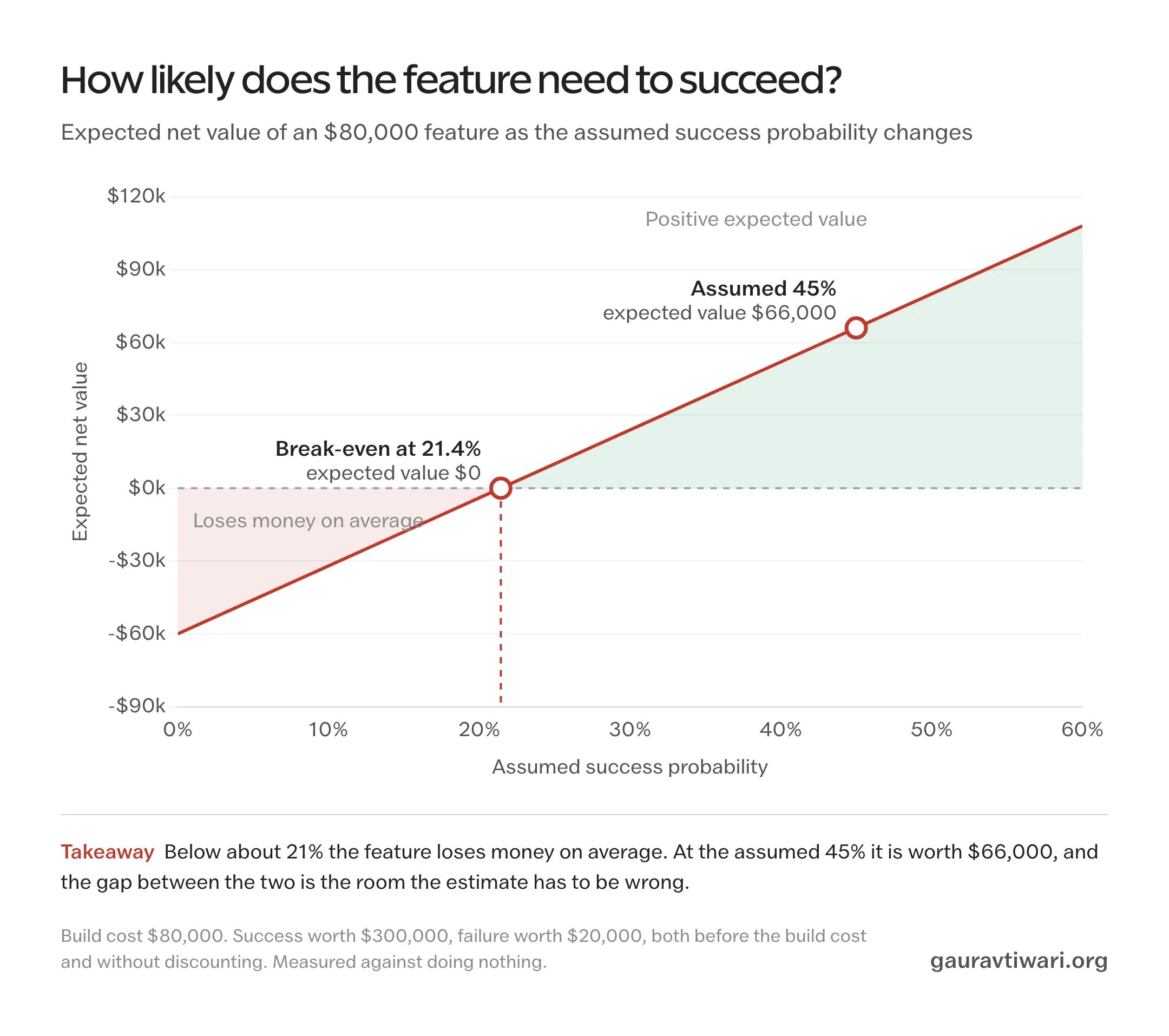
The threshold uses doing nothing as its baseline. A valuable alternative use of the same $80,000 raises the bar. I would compare that alternative too and check the evidence behind the probability estimate.

When Better Information Isn’t Worth Buying

The natural next move is to buy better information, say a $5,000 customer survey before building. Suppose the survey is right 80% of the time in both directions: 80% of features that test well succeed, and 80% of features that test poorly fail. Whether it is worth $5,000 depends on the whole strategy around it, not on the good result alone.

For a 45% base rate and an 80% accurate survey to hold together, a positive result has to come up 5 times in 12, about 42% of the time:

$$0.45 = 0.80\,q + 0.20\,(1-q) \quad \Rightarrow \quad q = \tfrac{5}{12}$$

With the survey result in hand, these are the moves on the table:

Decision after the survey	Expected feature payoff, before the survey fee
Build after a positive result	0.8 × $300,000 + 0.2 × $20,000 − $80,000 = $164,000
Build after a negative result	0.2 × $300,000 + 0.8 × $20,000 − $80,000 = −$4,000
Skip after a negative result	$0

So you build only after a positive result, and the survey route is worth:

$$\tfrac{5}{12}\,(\$164{,}000) – \$5{,}000 \approx \$63{,}333$$

Building without the survey was worth $66,000. Before its fee, the survey route is worth about $68,300, so the information adds about $2,300 in expected payoff, and it costs $5,000. Under these assumptions the survey lowers the expected payoff by about $2,700, even though it is exactly as accurate as promised. Better information is worth buying only when its expected improvement to the decision is bigger than its price, and you find that out by pricing the complete strategy rather than the favorable branch on its own.

When Positive Expected Value Isn’t Enough

I would check these limits before choosing an option just because its expected value is positive:

A Loss You Can’t Absorb

Two options can share an expected value and carry completely different risk. Option A pays $100,000 for certain. Option B pays $300,000 half the time and loses $100,000 the other half. Both have an expected value of $100,000, and only one of them can put you out of business.

A rare loss can dominate the practical decision. A 99% chance of gaining $200,000 and a 1% chance of losing $10 million has an expected value of $98,000. That positive average does not make the $10 million downside affordable. Expected value remains defined for a one-time choice, but you also need to judge its consequences. The guide to the mathematics of risk assessment discusses these risk questions, including sizing repeated decisions.

Inputs You Can’t Trust

An expected value can’t be more reliable than the probabilities that went into it, and a guessed probability is far more useful written down with its reasons than defended from memory. For every estimate that matters, record 5 things:

• the estimate itself
• where it came from: your own history, an industry base rate or a judgment call
• how many comparable cases sit behind it
• a plausible range, such as 35% to 55% rather than a flat 45%
• what new evidence would move it

“Six of ten similar proposals closed” is a useful observation, and it is still a sample of 10, which guarantees nothing about the next proposal. Uncertainty also lives outside the probabilities. Payoffs, costs, timing and the completeness of the scenario list can all be wrong, so the confidence you place in a calculation should follow the weakest of these inputs.

Multiplying separate probabilities gives their joint probability only when the events are independent. If product quality affects marketing success, that assumption may fail. Estimate the joint chance or use the appropriate conditional probabilities instead.

And recalculate when new evidence changes your probabilities or payoffs. A project that started at 60% can be an 80% project after 3 good months or a 40% one after a bad quarter, and the decision to continue should rest on the current number.

Things Money Doesn’t Measure

Expected value isn’t restricted to money. It works on hours, on units, on any outcome you can count. What it can’t do is weigh outcomes by how much they matter to you. A failed launch costs more than its dollar figure if it also costs a year of confidence, and a modest success can be worth more than its revenue if it opens a market. Expected utility is the version of the calculation that handles this. Each outcome passes through a utility function, a score for how much that outcome is worth to you, before it is weighted. It is more complete and more subjective, and it is the formal reason a cautious person can rationally turn down a bet with positive expected value.

Doors That Only Open One Way

A reversible choice gives you a chance to change course as you learn. For a hard-to-reverse decision, I would examine the downside before relying on a positive average. Jeff Bezos described this distinction as one-way and two-way doors in Amazon’s 2015 shareholder letter.

A Worksheet for Your Next Decision

A spreadsheet does this arithmetic better than a calculator, because the total updates the moment you change an assumption, which is the whole point of testing one. Put the probabilities in B2:B7 and the net outcomes in C2:C7, then:

=SUMPRODUCT(B2:B7,C2:C7)

SUMPRODUCT multiplies each probability by its outcome and adds the results, which is exactly the expected value formula. Enter probabilities as percentages, 10% rather than 10, and keep a separate cell that totals B2:B7 so you can see at a glance that the model adds up to 100%. The formula works the same way in Excel and in Google Sheets.

If you’d rather start from a finished sheet, the worksheet below has the launch example on its first tab, a break-even tab that works out the threshold and the sensitivity table from your own cost and value figures, a tab for comparing options and an estimate log. Change the yellow cells and everything else recalculates.

Then, before committing to anything, run through this list:

• the expected net result, with every cost counted once
• the chance of losing money, and the worst listed outcome
• whether you could absorb that worst outcome without it changing anything else you care about
• the break-even probability, and what evidence says you clear it
• the best alternative use of the same money and time, because that is the real baseline
• the one assumption that flips the answer if it turns out wrong

If one of those checks is unresolved, investigate it before committing. The calculation helps you identify which missing information could change the choice.

FAQs on Expected Value

Final Remarks

Before committing, I want to know the expected net result, the loss I might have to absorb and which assumptions could change the answer. I would use those together to judge the choice.

The worksheet above is yours to keep for the next decision. For practice, the expected value study notes on this site work through more examples, from a project bid to an insurance premium, and end with a 10-question practice set with full solutions. The PDF is free to download from that page.