Differential Equation

A differential equation is an equation that relates a function to its derivatives. They describe how things change, which makes them the natural language of physics, engineering, biology, economics, and essentially every quantitative field. Newton’s laws are differential equations. Maxwell’s equations are differential equations. Population dynamics, chemical reaction rates, electric circuits, heat flow, sound waves, financial derivatives, all start as differential equations. Solving them is what calculus, in a sense, is for.

What a Differential Equation Is

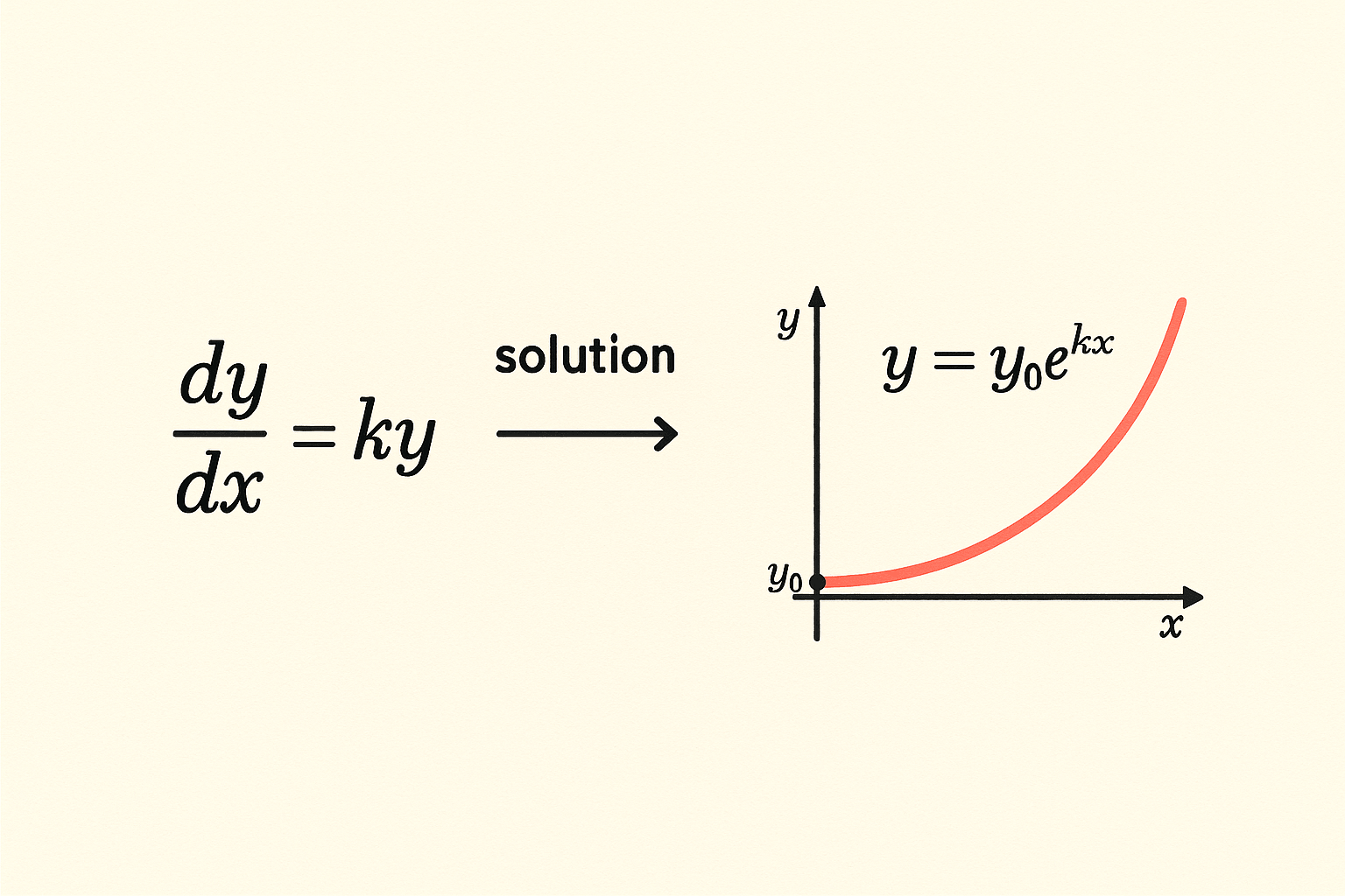
A differential equation contains derivatives of an unknown function. The simplest example:

$$ \frac{dy}{dx} = k y $$

This says: ‘the rate of change of \( y \) with respect to \( x \) is proportional to \( y \) itself.’ Solving it means finding the function \( y(x) \) that satisfies the equation. In this case, the solution is the exponential:

$$ y(x) = y_0 e^{kx} $$

where \( y_0 \) is the value of \( y \) at \( x = 0 \). You can verify by differentiating: \( dy/dx = k y_0 e^{kx} = k y \). ✓

Order and Linearity

Differential equations are classified by two main properties:

• Order = the highest derivative that appears. \( dy/dx = ky \) is first-order. \( d^2y/dx^2 + 4y = 0 \) is second-order. Newton’s second law \( F = m \\frac{d^2x}{dt^2} \) is also second-order.
• Linearity: a differential equation is LINEAR if the unknown function and its derivatives appear only to the first power and not multiplied together. Otherwise it’s nonlinear. Linear equations have nice properties (superposition, closed-form solutions, predictable behavior). Nonlinear equations are harder and can exhibit chaos.

Ordinary vs Partial

Two big subdivisions of the differential equation universe.

• Ordinary differential equations (ODEs) involve a single independent variable (usually time, often denoted t, or position, denoted x). The unknown is a function of one variable. Newton’s laws for a particle on a line are ODEs.
• Partial differential equations (PDEs) involve multiple independent variables. The unknown is a function of several variables, and derivatives are partial. The heat equation, wave equation, and Maxwell’s equations are PDEs. Much harder to solve in general.

Three Canonical First-Order ODEs

Exponential growth/decay

$$ \frac{dy}{dx} = k y \implies y(x) = y_0 e^{kx} $$

Models: bank interest, population growth, radioactive decay, drug elimination from the body, RC circuit discharge.

Logistic growth (population with carrying capacity)

$$ \frac{dy}{dx} = k y \left(1 – \frac{y}{K}\right) $$

Solution is an S-shaped curve approaching the carrying capacity \( K \). Models population dynamics under resource limits, technology adoption, epidemic spread (early phase), and many other ‘limit to growth’ phenomena.

Newton’s law of cooling

$$ \frac{dT}{dt} = -k (T – T_{env}) $$

The rate at which an object’s temperature \( T \) approaches the environment temperature \( T_{env} \) is proportional to the temperature difference. Solution is an exponentially decaying difference.

Second-Order: The Pendulum and Spring

Newton’s second law \( F = ma = m \\ddot{x} \) is naturally second-order. For a mass on a spring with restoring force \( F = -kx \):

$$ m \frac{d^2 x}{dt^2} = -kx \implies \frac{d^2 x}{dt^2} + \omega^2 x = 0 $$

where \( \\omega = \\sqrt{k/m} \). The general solution is \( x(t) = A \\cos(\\omega t) + B \\sin(\\omega t) \), or equivalently \( x(t) = C \\cos(\\omega t + \\varphi) \), simple harmonic motion. The same equation describes pendulums (small angles), LC circuits, and molecular vibrations.

Add damping (a friction-like term proportional to velocity) and the equation becomes \( \\ddot{x} + 2\\gamma \\dot{x} + \\omega^2 x = 0 \). The solutions depend on the damping ratio: under-damped (oscillates while decaying), critically damped (fastest return to rest without overshoot), or over-damped (slow exponential return). Critical damping is the design target for car shock absorbers and door closers.

Initial Conditions and Boundary Conditions

A differential equation has infinitely many solutions in general. To pick one specific solution, you need additional information.

• Initial conditions specify the function value (and possibly its derivatives) at one point. For first-order ODEs, you need 1 initial condition (e.g., \( y(0) = 5 \)). For second-order, 2 (e.g., \( x(0) = A \), \( \\dot{x}(0) = 0 \)).
• Boundary conditions specify values at multiple points (often the boundaries of the spatial domain for PDEs). E.g., the temperature at both ends of a metal rod.

An ODE plus its initial conditions is called an initial value problem (IVP); a PDE plus boundary conditions is a boundary value problem (BVP). Both have well-developed solution theories.

When You Can’t Solve Analytically

Most differential equations have no closed-form solution. For these, numerical methods take over. The basic idea: replace derivatives with finite differences and step through time computationally.

• Euler’s method: the simplest. Step forward by a small \( \Delta x \) using the current derivative. Fast but inaccurate.
• Runge-Kutta methods (RK4 in particular): much more accurate. The workhorse of numerical ODE solving.
• Adaptive methods: adjust step size based on local error estimates. What scipy.integrate.solve_ivp does by default.
• Finite element methods (FEM): for PDEs. Discretize the spatial domain into elements and solve the resulting algebraic system.

Modern computational physics and engineering depend completely on numerical differential equation solvers. Weather prediction, fluid dynamics simulations, structural analysis, drug pharmacokinetics, all are numerical PDE/ODE problems at the core.

Related study notes: Derivatives in Calculus, Exponential Function, Simple Harmonic Motion, Converting Differential to Integral Equations.

Practice Questions

Work each question before reading its solution. The set runs from direct recall and substitution to the applied questions that exams actually use to separate grades. All 10 also appear in the downloadable PDF with a separate answer key.

Question 1. What is a differential equation, and what does “solving” one actually produce?

Solution. An equation relating a function to its own derivatives, such as \(\frac{dy}{dx} = ky\). Solving it does not produce a number; it produces a FUNCTION, or a family of functions, that satisfies the relationship. The output of the whole exercise is a formula for how a quantity changes.

Question 2. Verify that \(y = 3e^{2x}\) solves \(\dfrac{dy}{dx} = 2y\).

Solution. \(\dfrac{dy}{dx} = 3 \cdot 2e^{2x} = 6e^{2x}\), and \(2y = 2(3e^{2x}) = 6e^{2x}\). They match at every \(x\), so the function satisfies the equation. Verification is just substitution, no solving skill required, which makes it the fastest way to check a proposed answer.

Question 3. Solve the separable equation \(\dfrac{dy}{dx} = \dfrac{x}{y}\).

Solution. Separate: \(y\,dy = x\,dx\). Integrate both sides: \(\frac{y^2}{2} = \frac{x^2}{2} + C\), so \(y^2 – x^2 = C\), a family of hyperbolas. Separable equations reduce calculus to 2 independent integrals, the most mechanical solving method available.

Question 4. Solve \(\dfrac{dy}{dx} = ky\) with initial condition \(y(0) = y_0\), and name the model it represents.

Solution. Separate and integrate: \(\ln y = kx + C\), so \(y = Ae^{kx}\); the initial condition fixes \(A = y_0\), giving \(y = y_0 e^{kx}\). This is exponential growth (\(k>0\)) or decay (\(k<0\)): population growth, radioactive decay, and compound interest are all this single equation with different signs and units.

Question 5. A radioactive isotope has a half-life of 10 years. Find its decay constant \(k\), and the fraction remaining after 25 years.

Solution. \(y = y_0 e^{kt}\) with \(y(10) = y_0/2\): \(e^{10k} = 0.5\), so \(k = \frac{\ln 0.5}{10} \approx -0.0693\)/yr. After 25 years: \(e^{-0.0693 \times 25} = e^{-1.733} \approx 0.177\), about 17.7% remains. Half-life problems are exponential decay with the constant reverse-engineered from a single data point.

Question 6. What is Newton’s law of cooling as a differential equation, and what does the constant \(k\) represent physically?

Solution. \(\dfrac{dT}{dt} = -k(T – T_{env})\): the cooling rate is proportional to how far the object’s temperature exceeds the surroundings. \(k\) bundles the object’s surface area, material, and heat-transfer efficiency; a larger \(k\) means faster equilibration. As \(T \to T_{env}\), the rate itself vanishes, which is why cooling curves flatten rather than crossing the ambient temperature.

Question 7. Coffee at 90°C cools in a 20°C room; after 10 minutes it is 60°C. Find its temperature after 20 minutes.

Solution. Solve \(T = T_{env} + (T_0 – T_{env})e^{-kt} = 20 + 70e^{-kt}\). At \(t=10\): \(40 = 70e^{-10k}\), so \(e^{-10k} = 4/7\). At \(t = 20\): \(e^{-20k} = (4/7)^2 = 16/49\), giving \(T = 20 + 70(16/49) \approx 42.9°\)C. Squaring the ratio for double the time is the shortcut once \(k\) itself is never needed explicitly.

Question 8. Solve the first-order linear equation \(\dfrac{dy}{dx} + 2y = 6\) using an integrating factor.

Solution. Integrating factor \(\mu = e^{\int 2\,dx} = e^{2x}\). Multiply through: \(\frac{d}{dx}(ye^{2x}) = 6e^{2x}\). Integrate: \(ye^{2x} = 3e^{2x} + C\), so \(y = 3 + Ce^{-2x}\). Every first-order linear equation surrenders to this 1 recipe: find \(\mu\), multiply, recognize a product rule, integrate.

Question 9. A tank holds 100 L of pure water. Brine with 2 g/L salt flows in at 5 L/min, and the well-mixed solution flows out at the same rate. Set up (do not fully solve) the differential equation for the salt amount \(S(t)\).

Solution. Rate in: \(2 \times 5 = 10\) g/min. Rate out: concentration times outflow, \(\frac{S}{100} \times 5 = \frac{S}{20}\) g/min. So \(\dfrac{dS}{dt} = 10 – \dfrac{S}{20}\). Mixing-tank problems are all “rate in minus rate out,” with the outflow rate always depending on the current amount, which is exactly what makes them differential rather than algebraic.

Question 10. Why do many differential equations, including most nonlinear ones, have no closed-form solution, and what do scientists do instead?

Solution. Only special structures, separable, linear, a handful of named forms, integrate into elementary functions; most equations describing real coupled systems (weather, orbits of 3+ bodies, epidemics with feedback) do not. Numerical methods (Euler’s method, Runge-Kutta) step forward in tiny increments, trading an exact formula for a highly accurate simulated curve, which is how modern climate and engineering models actually run.

Frequently Asked Questions

Browse more in Mathematics.