Gradient and Divergence

Gradient and divergence are vector-calculus operators that extract geometric information from scalar and vector fields. The gradient of a scalar field points in the direction of steepest increase and has magnitude equal to the rate of that increase. The divergence of a vector field measures the net outflow per unit volume at a point — how much the field ‘spreads out’ from there. Both are written with the nabla operator $ \nabla $ and are essential in fluid dynamics, electromagnetism, heat transfer, and any setting where quantities vary in space.

The Nabla Operator

The nabla or del operator is a formal vector of partial derivatives:

$$ \nabla = \left(\frac{\partial}{\partial x}, \frac{\partial}{\partial y}, \frac{\partial}{\partial z}\right) $$

Applied to a scalar field, it produces a vector (the gradient). Combined as a dot product with a vector field, it produces a scalar (the divergence). Combined as a cross product with a vector field, it produces another vector (the curl, beyond this note).

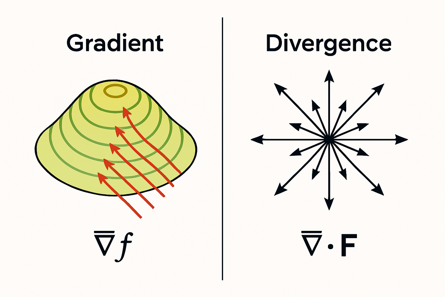
Gradient

For a scalar field $ f(x, y, z) $ (think temperature or elevation), the gradient is the vector:

$$ \nabla f = \left(\frac{\partial f}{\partial x}, \frac{\partial f}{\partial y}, \frac{\partial f}{\partial z}\right) $$

Direction: the gradient at a point is perpendicular to the level surface (or level curve) through that point and points ‘uphill’ — the direction of steepest increase.

Magnitude: equals the slope of the steepest ascent at that point. A flat region (constant $ f $) has gradient zero.

Example. $ f(x, y) = x^2 + y^2 $. $ \nabla f = (2x, 2y) $. At $ (1, 1) $, $ \nabla f = (2, 2) $ — pointing diagonally away from the origin. Makes sense: the function increases fastest in the direction away from the minimum.

Divergence

For a vector field $ \vec{F} = (F_x, F_y, F_z) $ (think fluid velocity or electric field), the divergence is the scalar:

$$ \nabla \cdot \vec{F} = \frac{\partial F_x}{\partial x} + \frac{\partial F_y}{\partial y} + \frac{\partial F_z}{\partial z} $$

Physical interpretation. $ \nabla \cdot \vec{F} $ at a point is the net outflow per unit volume from an infinitesimal box around the point.

Positive divergence: field is ‘spreading out’ (a source). Example: $ \vec{F} = (x, y, z) $ has $ \nabla \cdot \vec{F} = 3 > 0 $ — field radiates from the origin.
Negative divergence: field is converging (a sink).
Zero divergence: field is incompressible — what flows in flows out. Magnetic fields in classical electromagnetism have zero divergence everywhere (no magnetic monopoles).

Worked Example

$ \vec{F}(x, y, z) = (x^2, xy, z) $. Compute $ \nabla \cdot \vec{F} $.

$ \dfrac{\partial}{\partial x}(x^2) = 2x $, $ \dfrac{\partial}{\partial y}(xy) = x $, $ \dfrac{\partial}{\partial z}(z) = 1 $. So $ \nabla \cdot \vec{F} = 2x + x + 1 = 3x + 1 $. The divergence depends on position — varies linearly in $ x $.

Divergence Theorem

The divergence theorem (Gauss’s theorem) connects local and global behavior:

$$ \iiint_V (\nabla \cdot \vec{F})\, dV = \oiint_{\partial V} \vec{F} \cdot d\vec{A} $$

The total divergence inside a volume $ V $ equals the total flux out through its boundary surface. This is the precise mathematical statement of ‘what goes out must come from inside’.

Why They Matter

Electromagnetism. Two of Maxwell’s four equations involve divergence: ∇·E = ρ/ε₀ (charges are sources of electric field) and ∇·B = 0 (no magnetic monopoles).
Fluid dynamics. Continuity equation: ∂ρ/∂t + ∇·(ρv) = 0. Mass is conserved if outflow at a point matches the rate of density decrease. Incompressible fluids satisfy ∇·v = 0.
Heat transfer. The heat equation involves the Laplacian, which is the divergence of the gradient: ∂T/∂t = α ∇·(∇T) = α ∇²T.
Optimization and machine learning. Gradient descent updates parameters opposite to the gradient of a loss function. Every modern neural network is trained this way.
Topographic and physical maps. Contour lines on a map are level curves; gradient arrows point perpendicular to them and uphill.

Frequently Asked Questions

What is the gradient of a function?

The gradient ∇f of a scalar field f(x, y, z) is the vector of its partial derivatives: (∂f/∂x, ∂f/∂y, ∂f/∂z). It points in the direction of steepest increase of f and has magnitude equal to the rate of increase in that direction. It’s perpendicular to level surfaces of f.

What is divergence?

The divergence ∇·F of a vector field F is the scalar sum of its diagonal partial derivatives: ∂F_x/∂x + ∂F_y/∂y + ∂F_z/∂z. It measures the net outflow per unit volume at each point. Positive divergence means a source (field spreads out); negative means a sink; zero means flow is incompressible.

What does the symbol ∇ mean?

∇ is the ‘nabla’ or ‘del’ operator — a formal vector of partial derivatives. Applied to a scalar f, ∇f gives the gradient (a vector). Dotted with a vector field F, ∇·F gives the divergence (a scalar). Crossed with F, ∇×F gives the curl (a vector). It’s the central notation of vector calculus.

How is the gradient used in machine learning?

Gradient descent: to minimize a loss function L(θ) over model parameters θ, compute ∇L (the vector of partial derivatives), then take a small step in the direction −∇L. Repeating drives θ toward a local minimum. Backpropagation is the chain rule applied to compute ∇L efficiently for neural networks.

What is the divergence theorem?

Also called Gauss’s theorem. It states that the integral of the divergence of a vector field over a volume equals the flux of the field through the boundary surface: ∫∫∫ ∇·F dV = ∮∮ F·dA. It’s the higher-dimensional analogue of the fundamental theorem of calculus.

Why does ∇·B = 0 in electromagnetism?

Because no magnetic monopoles have ever been observed. Magnetic field lines always form closed loops — they don’t start or end anywhere. The mathematical expression of ‘no isolated magnetic charges’ is that the divergence of the magnetic field is zero everywhere. This is one of Maxwell’s equations.