Fundamental Theorem of Calculus

The Fundamental Theorem of Calculus (FTC) is the result that ties differentiation and integration together as inverse operations. Without it, integrals would still be limits of Riemann sums you’d compute by brute force. With it, you find an antiderivative and subtract two values. Done.

The FTC has two parts that look related but say different things. Both matter. Both deserve a minute of your time even if you’ve already memorized them. Together they form the most important theorem in single-variable calculus and the bridge between Newton-Leibniz era discoveries and modern analysis.

This study note covers both parts of the FTC, the intuition behind why they work, multiple worked examples, the connection to the mean value theorem, applications across science and engineering, common pitfalls, and the historical context that explains why this theorem changed mathematics.

Part 1: Derivative of an Integral

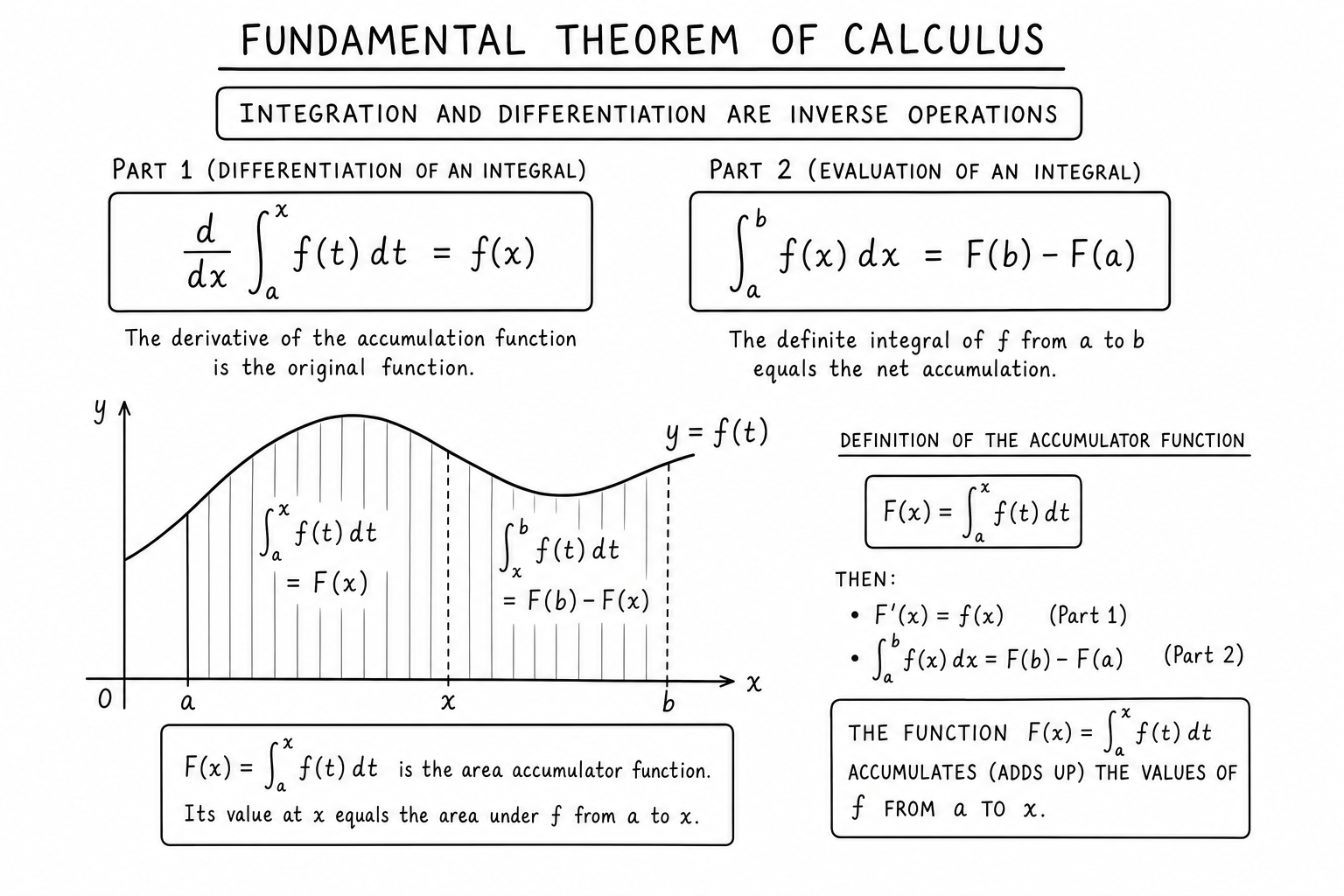
If \(f\) is continuous on \([a, b]\), define:

$$F(x) = \int_a^x f(t)\, dt$$

Then \(F\) is differentiable and:

$$F'(x) = f(x)$$

This says: integrating a continuous function and then differentiating recovers the original function. Differentiation undoes integration.

It also constructs antiderivatives: every continuous function has an antiderivative, given explicitly by an accumulator integral. This is a deep existence result. Even when you can’t write down the antiderivative in closed form, FTC Part 1 guarantees it exists as the integral function.

Part 2: Evaluating Definite Integrals

If \(F\) is any antiderivative of \(f\) on \([a, b]\) (i.e., \(F'(x) = f(x)\)), then:

$$\int_a^b f(x)\, dx = F(b) – F(a)$$

This is the workhorse. It turns a definite integral into a two-step calculation: find any antiderivative, plug in both endpoints, subtract. No Riemann sums required.

The shorthand \([F(x)]_a^b\) is universal in textbooks for the evaluation step. Some books use \(F(b) – F(a) = F\big|_a^b\). All the notations mean the same operation.

Worked Example: Polynomial

Compute \(\int_0^2 (3x^2 + 2x)\, dx\):

An antiderivative is \(F(x) = x^3 + x^2\). Apply Part 2:

$$\int_0^2 (3x^2 + 2x)\, dx = F(2) – F(0) = (8 + 4) – (0 + 0) = 12$$

That’s it. Three lines, no Riemann sums, no limits. The FTC is why integration in practice is just antidifferentiation plus subtraction.

Worked Example: Trig Integral

Compute \(\int_0^{\pi} \sin x\, dx\):

An antiderivative is \(F(x) = -\cos x\). Apply Part 2:

$$\int_0^{\pi} \sin x\, dx = (-\cos \pi) – (-\cos 0) = (1) – (-1) = 2$$

The integral of one full half-cycle of the sine curve equals 2. The geometric area between the curve and the x-axis from 0 to \(\pi\) is exactly 2 square units. This is how FTC turns geometry into arithmetic.

Worked Example: A Variable-Bound Integral

Find the derivative of \(F(x) = \int_1^{x^2} \sin(t^2)\, dt\).

This combines Part 1 with the chain rule. The upper bound is \(x^2\) (not just \(x\)), so use the chain rule:

$$F'(x) = \sin((x^2)^2) \cdot \frac{d}{dx}(x^2) = \sin(x^4) \cdot 2x = 2x \sin(x^4)$$

The integrand \(\sin(t^2)\) has no elementary antiderivative, so you can’t compute \(F(x)\) in closed form. But the FTC + chain rule still gives \(F'(x)\) cleanly. This is one of the deeper applications of Part 1 — derivatives of accumulator functions, even when the integrand resists symbolic integration.

Why It Works (Intuition)

Imagine \(f(x)\) is a velocity function. The integral \(\int_a^b f(x)\, dx\) is the total distance traveled from time \(a\) to \(b\). If \(F(x)\) is position, then \(F'(x) = f(x)\) (velocity is the derivative of position). Total distance = final position − initial position = \(F(b) – F(a)\).

That’s the FTC in one sentence. The two views — accumulating rate over time vs measuring change in the underlying quantity — describe the same thing. The theorem just makes that exact.

Part 1 has a parallel intuition. Define \(F(x)\) as the area under the curve from \(a\) to \(x\). When \(x\) increases by a tiny amount \(\Delta x\), the area increases by approximately \(f(x) \cdot \Delta x\) — a thin rectangle of width \(\Delta x\) and height \(f(x)\). So \(F'(x) = f(x)\). Areas grow at the rate the curve sits at.

Connection to the Mean Value Theorem for Integrals

If \(f\) is continuous on \([a, b]\), there exists \(c \in (a, b)\) such that:

$$\int_a^b f(x)\, dx = f(c)(b – a)$$

This is the Mean Value Theorem for Integrals. It says the integral equals the integrand evaluated at some interior point times the interval width — geometrically, there’s always a horizontal line at height \(f(c)\) that gives a rectangle with the same area as the integral.

The MVT for integrals follows from the FTC and the standard MVT (for derivatives). Together they form the calculus of “average behavior”: the average value of \(f\) on \([a, b]\) is \(\frac{1}{b-a}\int_a^b f(x)\, dx\), and the MVT guarantees this average is achieved somewhere in the interval.

Why FTC Is the Most Important Theorem in Calculus

• It makes integration tractable. Without it, every definite integral requires a Riemann limit calculation.
• It guarantees existence of antiderivatives for continuous functions.
• It unifies the two threads of calculus into one structure.
• It’s the bridge to differential equations, the divergence theorem, Stokes’ theorem, and most of higher-dimensional analysis.
• It’s the algebraic backbone for the Riemann integral and most of classical analysis.

Newton and Leibniz independently arrived at it in the 1670s, which is why it’s sometimes called the Newton-Leibniz formula. Read more in Aryabhata’s contributions to mathematics and interesting math articles and must-read research papers.

Generalizations: Stokes’ Theorem and Beyond

The FTC generalizes to higher dimensions and broader settings. Each generalization preserves the same fundamental insight: integrating a derivative over a region equals the difference of values on the boundary.

• Green’s Theorem: relates a line integral around a closed curve to a double integral over the region it encloses.
• Stokes’ Theorem: relates a surface integral of curl to a line integral around the boundary curve.
• Divergence Theorem (Gauss): relates a volume integral of divergence to a surface integral over the boundary.
• General Stokes’ Theorem: for differential forms on manifolds, \(\int_M d\omega = \int_{\partial M} \omega\). All the above are special cases.

This structural identity — boundary integral equals interior integral of the derivative — is one of the deepest patterns in mathematics. It appears in physics (Maxwell’s equations in differential form), engineering (finite element methods), and topology (de Rham cohomology).

Common Pitfalls

1. Forgetting absolute value when integrating \(1/x\). The antiderivative is \(\ln|x| + C\). The FTC then needs careful handling when the interval crosses zero.
2. Applying the FTC across discontinuities. The FTC requires \(f\) to be continuous on \([a, b]\). If \(f\) blows up inside the interval, treat the integral as improper and split at the discontinuity.
3. Using a wrong antiderivative. Any antiderivative works for Part 2, but it must actually satisfy \(F’ = f\) on the entire interval. Mismatched antiderivatives produce wrong answers.
4. Confusing the two parts. Part 1 says differentiating an integral recovers the integrand. Part 2 says evaluating a definite integral uses antiderivatives. Different statements, often conflated.
5. Not using the chain rule for variable-bound integrals. When the upper bound is \(g(x)\) instead of just \(x\), the derivative needs the chain rule: \(\frac{d}{dx} \int_a^{g(x)} f(t)\, dt = f(g(x)) \cdot g'(x)\).

Where the FTC Shows Up in Practice

• Physics: evaluating work, energy, impulse, and most quantities defined as accumulations over time or space.
• Probability: connecting cumulative distribution functions to probability density functions. The PDF is the derivative of the CDF; the CDF is an integral of the PDF.
• Engineering: stress and strain integrations, fluid flow accumulations, signal energy calculations.
• Economics: consumer surplus and producer surplus from integrating supply and demand curves.
• Numerical methods: the FTC justifies that numerical integration converges to the same value as exact integration, validating finite-element and finite-difference techniques.
• Differential equations: nearly every solution technique invokes the FTC at some step to translate between rate and accumulation.

History and Modern Significance

James Gregory and Isaac Barrow developed pieces of the FTC in the mid-1600s. Newton and Leibniz independently formulated and exploited the full result in the 1670s. The FTC was the discovery that turned calculus from a collection of clever tricks into a unified theory.

The 18th and 19th centuries developed the rigorous foundations. Cauchy and Riemann formalized integration; Weierstrass formalized derivatives. By the late 19th century, the FTC had its modern epsilon-delta proof and its central place in analysis.

The 20th century generalized the FTC to differential forms on manifolds, where it becomes the general Stokes’ theorem. The 21st century continues to find applications in computer-aided geometry, numerical PDE solvers, and theoretical physics. Few results in mathematics have remained as central or as widely applied for so long.

FTC and Differential Equations

Many differential equations are solved by integrating both sides — directly invoking the FTC. For a separable equation \(dy/dx = f(x) g(y)\), separate variables and integrate: \(\int 1/g(y)\, dy = \int f(x)\, dx + C\). The FTC justifies that this integration produces a valid solution.

First-order linear equations \(y’ + p(x) y = q(x)\) use an integrating factor \(\mu(x) = \exp(\int p(x)\, dx)\), which makes the left side an exact derivative \((\mu y)’\), reducing the problem to one final integration. The FTC underwrites every step.

FTC in Probability and CDFs

For a continuous random variable with PDF \(f\) and CDF \(F\), the FTC says \(F'(x) = f(x)\) (Part 1) and \(\int_a^b f(x)\, dx = F(b) – F(a) = P(a \le X \le b)\) (Part 2). PDFs and CDFs are derivative–integral pairs related exactly through the FTC.

This connection is essential in statistics. Quantile-quantile plots, hazard functions, and survival analysis all rely on differentiating CDFs and integrating PDFs interchangeably.

FTC and the Method of u-Substitution

Substitution in definite integrals uses the FTC implicitly. When you substitute \(u = g(x)\), the new bounds are \(g(a)\) and \(g(b)\), and the integral becomes \(\int_{g(a)}^{g(b)} f(u)\, du\). Evaluating with the FTC gives \(F(g(b)) – F(g(a))\), which equals the original integral \((F \circ g)(b) – (F \circ g)(a)\) — exactly what FTC Part 2 applied directly would give.

So substitution is consistent with the FTC, not a separate trick layered on top. The whole apparatus of techniques of integration is essentially the FTC plus algebraic manipulation.

FTC in Vector Calculus: The Gradient Theorem

The gradient theorem (sometimes called the FTC for line integrals) says: for a smooth scalar function \(f\) and a smooth curve \(C\) from point \(\mathbf{a}\) to point \(\mathbf{b}\),

$$\int_C \nabla f \cdot d\mathbf{r} = f(\mathbf{b}) – f(\mathbf{a})$$

This is the direct multivariable analogue of FTC Part 2. The integral of a gradient along a path equals the difference of the function at the endpoints. It immediately implies that line integrals of conservative vector fields are path-independent.

From here, the generalization runs through Green’s theorem, Stokes’ theorem, and the divergence theorem to the full Stokes’ theorem on differential forms.

Worked Example: Computing a Definite Integral with FTC

Compute \(\int_1^4 (x^2 + 1)\, dx\). Antiderivative: \(F(x) = x^3/3 + x\). Apply FTC Part 2:

$$\int_1^4 (x^2 + 1)\, dx = F(4) – F(1) = \left(\frac{64}{3} + 4\right) – \left(\frac{1}{3} + 1\right) = 21 + 3 = 24$$

Three steps: find antiderivative, plug in upper bound, subtract lower-bound value. The FTC turns area-under-curve calculation into routine arithmetic.

Generalizations to Curves, Surfaces, and Volumes

The FTC’s structural identity — boundary integral equals interior integral of the derivative — generalizes across dimensions:

• Single-variable FTC: \(\int_a^b F’\, dx = F(b) – F(a)\).
• Gradient theorem: \(\int_C \nabla f \cdot d\mathbf{r} = f(\mathbf{b}) – f(\mathbf{a})\).
• Stokes’ theorem: \(\int_S (\nabla \times \mathbf{F}) \cdot d\mathbf{S} = \oint_{\partial S} \mathbf{F} \cdot d\mathbf{r}\).
• Divergence theorem: \(\int_V (\nabla \cdot \mathbf{F})\, dV = \oint_{\partial V} \mathbf{F} \cdot d\mathbf{S}\).
• General Stokes’ on differential forms: \(\int_M d\omega = \int_{\partial M} \omega\).

All five say the same conceptual thing in increasing generality. The FTC isn’t just a single theorem — it’s a pattern that recurs throughout multivariable calculus, vector analysis, and differential geometry.

FTC as the Bridge Between Integration and Differentiation

Before the FTC was understood, computing integrals required Riemann-sum-style limit arguments — slicing the area under a curve into thin rectangles, summing them, and taking a limit. This worked but was tedious for any but the simplest functions.

After Newton and Leibniz, the FTC reduced integration to antidifferentiation. Find any function whose derivative gives the integrand, and the integral is just an arithmetic difference. This shift from limits-of-sums to algebraic antidifferentiation is what made calculus practical and accessible to engineers, scientists, and economists.

The FTC also opens a productive feedback loop: integration tables grow as people discover new antiderivatives; antidifferentiation techniques (substitution, parts, partial fractions) translate the table into more usable forms; symbolic computation extends both. Today’s calculus toolbox is the cumulative result of three centuries of FTC-driven antiderivative discovery.

FTC and Numerical Integration

Numerical integration approximates definite integrals when no closed-form antiderivative exists. The trapezoidal rule, Simpson’s rule, and Gaussian quadrature all produce approximations that converge to the exact integral by the FTC.

The FTC also justifies adaptive integration schemes: refine sub-intervals where the function changes quickly, leave sub-intervals coarse where it changes slowly. Modern scientific computing relies heavily on these adaptive methods to handle integrals from physics simulations, financial models, and machine learning posterior inference.

Worked Example: Average Value via FTC

The average value of \(f\) on \([a, b]\) is \(\bar{f} = \frac{1}{b-a}\int_a^b f(x)\, dx\). For \(f(x) = x^2\) on \([0, 3]\):

$$\bar{f} = \frac{1}{3 – 0} \int_0^3 x^2\, dx = \frac{1}{3} \cdot \left[\frac{x^3}{3}\right]_0^3 = \frac{1}{3} \cdot 9 = 3$$

The average value is 3, computed using the FTC to evaluate the integral and then dividing by the interval width. The Mean Value Theorem for Integrals guarantees \(f(c) = 3\) for some \(c \in (0, 3)\); solving \(c^2 = 3\) gives \(c = \sqrt{3} \approx 1.732\), which is indeed inside the interval.

FAQs