Integrals in Calculus

Integrals in calculus accumulate quantities over intervals. Geometrically, the definite integral is the signed area between a curve and the x-axis. Physically, it turns rate into total: integrating velocity gives distance, integrating power gives energy, integrating probability density gives probability. Anywhere a continuous quantity adds up over a span, integrals are the math.

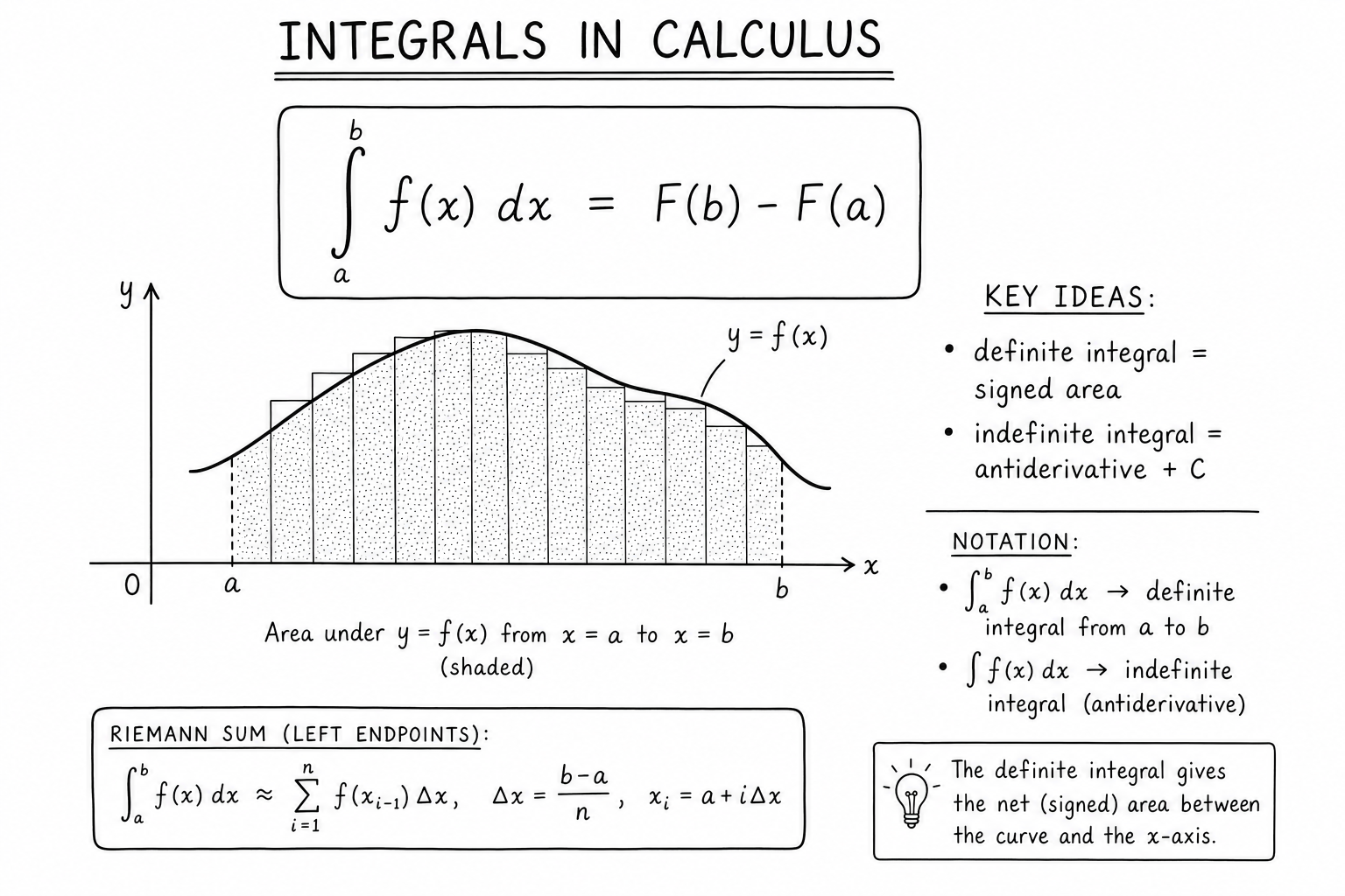
There are two species: definite integrals (numerical area between bounds) and indefinite integrals (families of antiderivatives). The Fundamental Theorem of Calculus connects them, which is why integration and differentiation are inverse operations. Once you’ve mastered the techniques, integrals turn what looked like impossible accumulations into one-line antiderivative lookups.

This study note covers the definitions, the Riemann sum foundation, standard antiderivatives, the four major integration techniques, applications across science and engineering, common pitfalls, numerical methods, and the historical and modern context.

Definite vs Indefinite Integrals

The indefinite integral is a family of antiderivatives:

$$\int f(x)\, dx = F(x) + C$$

where \(F'(x) = f(x)\) and \(C\) is the constant of integration.

The definite integral is a number — the signed area under \(f\) from \(a\) to \(b\):

$$\int_a^b f(x)\, dx = F(b) – F(a)$$

One is a function (plus a constant). The other is a number. Don’t drop the bounds and don’t drop the \(+ C\) — those are the two most common notation mistakes that haunt every introductory calculus class.

The Riemann Sum Definition

The definite integral is the limit of a Riemann sum:

$$\int_a^b f(x)\, dx = \lim_{n \to \infty} \sum_{i=1}^{n} f(x_i^*) \Delta x$$

Slice \([a, b]\) into \(n\) sub-intervals of width \(\Delta x = (b-a)/n\). For each sub-interval pick a sample point \(x_i^*\). Add up the rectangle areas \(f(x_i^*) \Delta x\). As \(n \to \infty\), the sum approaches the exact area.

This is what integrals are at the foundation. Every integration technique is just an efficient shortcut around the Riemann sum. Different choices of \(x_i^*\) (left endpoint, right endpoint, midpoint) give different finite-sample estimates but converge to the same limit for continuous functions.

Standard Antiderivatives

Memorize these and the table covers most of what comes up in coursework:

• \(\int x^n\, dx = \frac{x^{n+1}}{n+1} + C\) for \(n \neq -1\)
• \(\int \frac{1}{x}\, dx = \ln|x| + C\)
• \(\int e^x\, dx = e^x + C\)
• \(\int a^x\, dx = \frac{a^x}{\ln a} + C\)
• \(\int \sin x\, dx = -\cos x + C\)
• \(\int \cos x\, dx = \sin x + C\)
• \(\int \sec^2 x\, dx = \tan x + C\)
• \(\int \frac{1}{1+x^2}\, dx = \arctan x + C\)
• \(\int \frac{1}{\sqrt{1-x^2}}\, dx = \arcsin x + C\)

These are the essentials. A few more (hyperbolic functions, special quotients) round out the standard table that appears on the back cover of most calculus textbooks.

Integration Technique 1: Substitution

Substitution is the reverse of the chain rule. Let \(u = g(x)\), then \(du = g'(x)\, dx\). Rewrite the integral in terms of \(u\):

$$\int f(g(x)) g'(x)\, dx = \int f(u)\, du$$

Worked example: compute \(\int 2x \cos(x^2)\, dx\). Let \(u = x^2\), so \(du = 2x\, dx\). The integral becomes \(\int \cos u\, du = \sin u + C = \sin(x^2) + C\).

For definite integrals, change the bounds when you change variables: if \(u = g(x)\), the new bounds are \(g(a)\) and \(g(b)\). Substitution handles a huge fraction of textbook integrals; spot a function and its derivative both present, and substitution usually closes the case.

Integration Technique 2: Integration by Parts

Integration by parts is the reverse of the product rule:

$$\int u\, dv = uv – \int v\, du$$

Use it when the integrand is a product where one factor simplifies under differentiation (logs, polynomials, inverse trig functions) and the other is easy to integrate (exponentials, sines, cosines).

The mnemonic LIATE helps pick \(u\) (the factor to differentiate): Logarithmic, Inverse trig, Algebraic, Trigonometric, Exponential — choose whichever appears earliest in this list.

Worked example: \(\int x e^x\, dx\). Let \(u = x\) (algebraic, earlier in LIATE) and \(dv = e^x\, dx\). Then \(du = dx\) and \(v = e^x\). The formula gives \(\int x e^x\, dx = x e^x – \int e^x\, dx = x e^x – e^x + C = (x – 1) e^x + C\).

Integration Technique 3: Partial Fractions

For rational functions \(P(x)/Q(x)\) where \(\deg P < \deg Q\), decompose into simpler fractions, then integrate each piece using standard antiderivatives.

For \(\int \frac{1}{x^2 – 1}\, dx\), factor: \(x^2 – 1 = (x-1)(x+1)\). Decompose:

$$\frac{1}{(x-1)(x+1)} = \frac{A}{x-1} + \frac{B}{x+1}$$

Solving: \(A = 1/2\), \(B = -1/2\). Then \(\int \frac{1}{x^2 – 1}\, dx = \frac{1}{2} \ln|x-1| – \frac{1}{2} \ln|x+1| + C\).

Partial fractions handle integrals from quotient-of-polynomials cases that show up everywhere in differential equations and Laplace transform inversions. Modern computer algebra systems do the decomposition automatically; understanding the technique is still essential for clean by-hand work.

Integration Technique 4: Trigonometric Substitution

For integrals containing \(\sqrt{a^2 – x^2}\), \(\sqrt{a^2 + x^2}\), or \(\sqrt{x^2 – a^2}\), substitute trig identities to simplify:

• \(\sqrt{a^2 – x^2}\): let \(x = a \sin\theta\), so \(\sqrt{a^2 – x^2} = a \cos\theta\).
• \(\sqrt{a^2 + x^2}\): let \(x = a \tan\theta\), so \(\sqrt{a^2 + x^2} = a \sec\theta\).
• \(\sqrt{x^2 – a^2}\): let \(x = a \sec\theta\), so \(\sqrt{x^2 – a^2} = a \tan\theta\).

The trig substitution cleans up the radical and turns the integral into one involving only trig functions, which the standard antiderivative table handles. After integrating, substitute back from \(\theta\) to \(x\) using a right triangle diagram.

Trigonometric integrals also have their own family of identities (half-angle, product-to-sum, power reduction) that simplify integrands with high powers of sin and cos.

What Integrals Compute

• Area between a curve and an axis or between two curves.
• Volume of solids of revolution (disk, washer, shell methods).
• Arc length: \(L = \int_a^b \sqrt{1 + (f'(x))^2}\, dx\).
• Surface area of solids of revolution.
• Average value of a function over an interval: \(\bar{f} = \frac{1}{b-a}\int_a^b f(x)\, dx\).
• Total accumulation: distance from velocity, work from force, mass from density, charge from current.
• Probability from probability density: \(P(a < X < b) = \int_a^b f(x)\, dx\).
• Moments and centers of mass: \(\bar{x} = \frac{1}{M} \int x \rho(x)\, dx\).

Integrals show up everywhere in data science, business statistics (cumulative distribution functions are integrals of densities), and risk assessment.

Improper Integrals

An improper integral has either an infinite interval or an unbounded integrand:

$$\int_1^\infty \frac{1}{x^2}\, dx = \lim_{b \to \infty} \int_1^b \frac{1}{x^2}\, dx = \lim_{b \to \infty} \left[-\frac{1}{x}\right]_1^b = 1$$

The integral converges to 1. By contrast:

$$\int_1^\infty \frac{1}{x}\, dx = \lim_{b \to \infty} \ln b = \infty$$

diverges. The p-test summarizes the pattern: \(\int_1^\infty 1/x^p\, dx\) converges if and only if \(p > 1\).

Improper integrals appear constantly in probability (the integral of a density over the whole real line must equal 1), in physics (escape velocity calculations), and in engineering (response of systems to long-duration inputs).

Numerical Integration

Many integrals don’t have closed-form antiderivatives. Numerical methods estimate them by sampling the integrand:

• Trapezoidal rule: approximate the integral by trapezoids. Error scales as \(O(h^2)\) where \(h\) is the sample spacing.
• Simpson’s rule: use parabolic arcs through three consecutive points. Error scales as \(O(h^4)\) — much faster convergence.
• Gaussian quadrature: place sample points strategically to maximize accuracy for polynomial integrands. Standard tool in finite element analysis.
• Monte Carlo integration: sample the integrand at random points and average. Slow convergence (\(O(1/\sqrt{n})\)) but scales well to high dimensions.

Modern scientific computing relies heavily on numerical integration. The integrals arising in finance, physics simulation, and machine learning posterior inference are usually intractable analytically and demand numerical methods.

Common Pitfalls When Integrating

1. Dropping the constant of integration. Indefinite integrals always carry \(+ C\). Forgetting it loses a family of solutions and breaks differential equation work.
2. Misapplying the power rule. The formula fails when \(n = -1\) (then the antiderivative is \(\ln|x|\), not \(x^0/0\)). The exception is the most-tested edge case.
3. Forgetting absolute value in \(\int 1/x\, dx\). The antiderivative is \(\ln|x| + C\), not \(\ln x + C\) — the function is defined for all nonzero \(x\), not just positive \(x\).
4. Mixing up bounds in substitution. When changing variables in a definite integral, change the bounds to match the new variable. Or change back to the original variable before evaluating.
5. Ignoring discontinuities inside the interval. If the integrand blows up between the bounds, the integral is improper and needs to be split and treated as a limit.

History and Modern Use

The geometric idea behind integration is ancient: Eudoxus and Archimedes computed areas using the method of exhaustion in the 4th and 3rd centuries BCE. Cavalieri formalized “indivisibles” in the 17th century. Newton and Leibniz independently developed integral calculus in the 1670s and 1680s, recognizing that integration and differentiation are inverse operations — the Fundamental Theorem of Calculus.

Cauchy and Riemann put integration on rigorous footing in the 19th century. The Riemann integral handles continuous functions cleanly. The Lebesgue integral (1902) extends the theory to far broader function classes and is the standard in modern analysis and probability. Most undergraduate calculus courses still teach the Riemann version because it suffices for nearly every applied problem.

The 20th and 21st centuries shifted integration from a paper-and-pencil discipline to a computational one. Symbolic integration in computer algebra systems (Mathematica, SymPy) handles textbook integrals automatically. Numerical libraries (SciPy, NAG, GSL) handle integrals from real applications efficiently. Automatic integration is now invisibly woven into nearly every scientific computing workflow.

Lebesgue Integration vs Riemann Integration

The Riemann integral, taught in introductory calculus, partitions the domain (x-axis) into pieces. The Lebesgue integral partitions the range (y-axis) into pieces and asks how much of the domain maps to each y-band. The two integrals agree on continuous functions but Lebesgue handles discontinuous and pathological cases that Riemann can’t.

The Dirichlet function (1 on rationals, 0 on irrationals) isn’t Riemann integrable but is Lebesgue integrable with value 0. Modern probability theory, Fourier analysis, and functional analysis are built on the Lebesgue integral because it has cleaner convergence properties (dominated convergence, monotone convergence) than the Riemann integral.

Integration in Probability and Statistics

A continuous random variable’s probability density function (PDF) integrates to 1. The cumulative distribution function (CDF) is the integral of the PDF up to a point: \(F(x) = \int_{-\infty}^x f(t)\, dt\). Probabilities for ranges are integrals: \(P(a < X < b) = \int_a^b f(x)\, dx\).

Expected value uses an integral: \(E[X] = \int x f(x)\, dx\). Variance, higher moments, and characteristic functions are all integrals. Maximum likelihood estimation maximizes integrals (or sums for discrete data) of log-likelihood.

Multiple Integrals

Double integrals \(\iint_R f(x, y)\, dA\) compute volumes under surfaces over a 2D region. Triple integrals \(\iiint_V f(x, y, z)\, dV\) compute integrals over 3D volumes — used for mass, charge, moment of inertia.

Iterated integration evaluates multiple integrals one variable at a time. Fubini’s theorem says (under reasonable conditions) the order of integration doesn’t matter. For complex regions, change of variables (polar, cylindrical, spherical, or general) introduces a Jacobian factor that adjusts for the coordinate transformation. The change-of-variable formula is a multivariable application of the chain rule.

Improper Integrals and Convergence Tests

The p-test: \(\int_1^\infty 1/x^p\, dx\) converges if and only if \(p > 1\), and \(\int_0^1 1/x^p\, dx\) converges if and only if \(p < 1\). These two cases cover most textbook improper integrals.

Comparison test: if \(0 \le f(x) \le g(x)\) for large \(x\), and \(\int g\, dx\) converges, then \(\int f\, dx\) converges. If \(\int f\, dx\) diverges, so does \(\int g\, dx\). Limit comparison test compares the ratio \(f(x)/g(x)\). These tests are the analytic counterparts of series convergence tests and are used routinely in advanced calculus.

Worked Example: Volume of a Sphere

The volume of a sphere of radius \(R\) is computed by integrating the cross-sectional area along an axis. At height \(y\) from the center, the cross-section is a circle of radius \(\sqrt{R^2 – y^2}\) and area \(\pi (R^2 – y^2)\).

$$V = \int_{-R}^R \pi (R^2 – y^2)\, dy = \pi \left[R^2 y – \frac{y^3}{3}\right]_{-R}^R = \frac{4}{3}\pi R^3$$

This is the standard derivation of the famous formula. Other rotational solids, irregular volumes, and surfaces of revolution all follow the same template: identify cross-sections, compute area, integrate along the axis.

Integration in Engineering

Engineers integrate constantly. Stress-strain curves get integrated to compute strain energy. Velocity profiles get integrated to compute flow rates. Power dissipation over time gets integrated to compute total energy. Probability density of failure times gets integrated to compute reliability functions.

Finite element analysis software automates these integrations across millions of mesh elements. The math behind each element is plain calculus integration; the engineering breakthrough is doing it efficiently across complex 3D geometries with millions of degrees of freedom.

Integration by Parts: Choosing u and dv

Integration by parts works only when you pick the right \(u\) and \(dv\). The LIATE mnemonic is the standard heuristic: choose \(u\) as the factor that appears earliest in the list Logarithmic, Inverse trig, Algebraic, Trigonometric, Exponential. The remaining piece becomes \(dv\).

Why this works: \(u\) gets differentiated, so picking the factor that simplifies under differentiation makes the resulting integral easier. Logarithms become rational functions; polynomials become lower-degree polynomials; inverse trig functions become algebraic. Exponentials and trig functions don’t simplify, so they’re chosen for \(dv\).

Sometimes integration by parts has to be applied repeatedly. The classic example: \(\int x^2 e^x\, dx\) requires two applications, with the polynomial degree dropping by one each time. After two iterations the polynomial is gone and the integral closes cleanly.

Improper Integrals: Worked Example

Compute \(\int_0^\infty e^{-x}\, dx\). This is improper because the upper bound is infinite. Treat it as a limit:

$$\int_0^\infty e^{-x}\, dx = \lim_{b \to \infty} \int_0^b e^{-x}\, dx = \lim_{b \to \infty} (1 – e^{-b}) = 1$$

The integral converges to 1. This particular result is the normalization for the exponential probability distribution and shows up constantly in applied math.

FAQs