Determinants

Determinants in linear algebra are scalar values computed from square matrices that capture how the matrix scales volumes (or signed volumes) under its corresponding linear transformation. Despite their simple-looking definition, determinants encode a remarkable amount of structural information about a matrix: invertibility, orientation, eigenvalue products, and more.

If the determinant is zero, the matrix is singular — its columns are linearly dependent and it has no inverse. If the determinant is positive, the transformation preserves orientation; if negative, it flips orientation. The absolute value tells you the scaling factor for volumes. These three pieces of information are why determinants appear so often in matrix analysis.

This study note covers the 2×2 formula, cofactor expansion for larger matrices, the geometric interpretation, the standard properties, the connection to invertibility, applications, common pitfalls, and a brief history.

The 2×2 Formula

For a 2×2 matrix:

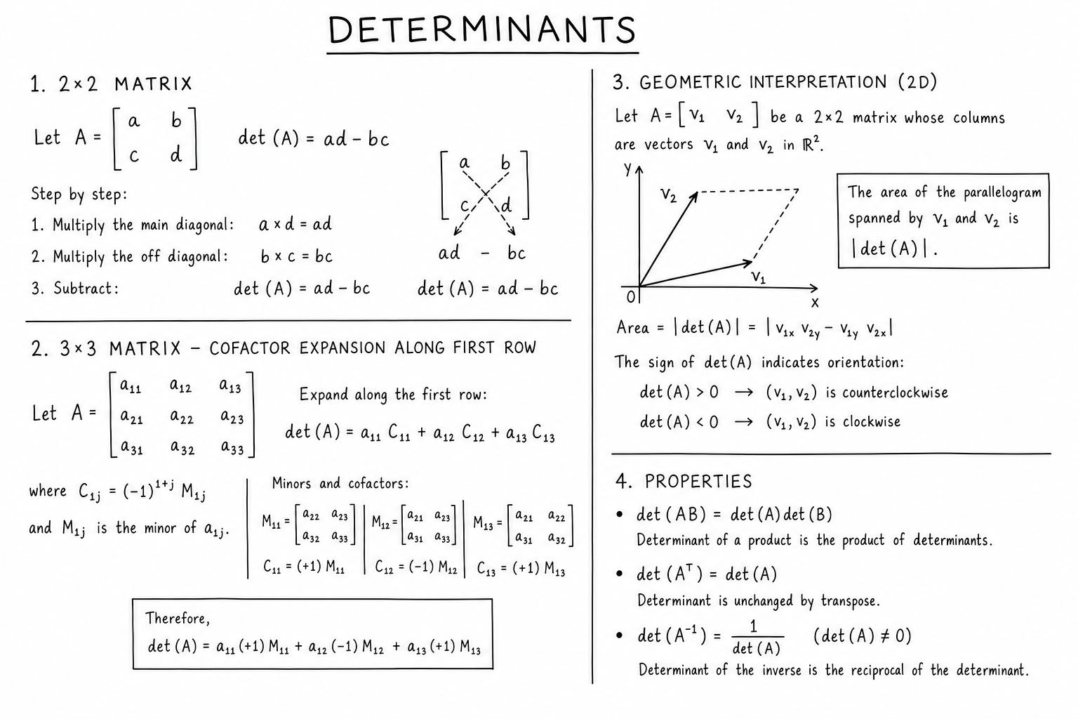
$$\det \begin{pmatrix} a & b \\ c & d \end{pmatrix} = ad – bc$$

This is the simplest case. Multiply the diagonal entries, subtract the product of the off-diagonal entries. Easy to compute, easy to remember.

Geometrically, this equals the signed area of the parallelogram with sides given by the column vectors \((a, c)\) and \((b, d)\). The sign indicates orientation: positive if the vectors are in counterclockwise order, negative if clockwise.

The 3×3 Formula and Cofactor Expansion

For a 3×3 matrix:

$$\det A = a_{11}(a_{22}a_{33} – a_{23}a_{32}) – a_{12}(a_{21}a_{33} – a_{23}a_{31}) + a_{13}(a_{21}a_{32} – a_{22}a_{31})$$

This is cofactor expansion along the first row. Each entry \(a_{1j}\) is multiplied by the determinant of the 2×2 matrix obtained by deleting row 1 and column \(j\), with alternating signs.

Cofactor expansion generalizes to any \(n \times n\) matrix:

$$\det A = \sum_{j=1}^n (-1)^{1+j} a_{1j} M_{1j}$$

where \(M_{1j}\) is the determinant of the (n−1)×(n−1) submatrix obtained by deleting row 1 and column \(j\). You can expand along any row or column; the answer is the same.

Geometric Interpretation

The determinant of an \(n \times n\) matrix equals the signed volume of the parallelepiped spanned by its column vectors. In 2D, that’s a parallelogram area. In 3D, it’s a parallelepiped volume. In higher dimensions, the same idea extends to “hypervolume” measured in n-dimensional units.

The sign indicates orientation. In 3D, positive determinant means the columns form a right-handed coordinate system; negative means left-handed. This is why determinants appear in change-of-variable formulas in multivariable calculus — the absolute value adjusts for the volume scaling, and the sign tracks orientation.

A determinant of zero means the columns are linearly dependent and the parallelepiped is degenerate (collapsed to lower dimension, with zero volume). This is the geometric meaning of singularity.

Properties

• \(\det(I) = 1\). The identity preserves volumes.
• \(\det(AB) = \det(A)\det(B)\). The product rule.
• \(\det(A^T) = \det(A)\). Transpose preserves determinant.
• \(\det(A^{-1}) = 1/\det(A)\). Inverses divide.
• \(\det(cA) = c^n \det(A)\) for an \(n \times n\) matrix. Scalars scale every row.
• Swapping two rows changes the sign of the determinant.
• Adding a multiple of one row to another doesn’t change the determinant.
• Multiplying a row by \(c\) multiplies the determinant by \(c\).

The last three properties are the engine behind row-reduction-based determinant computation. They let you reduce a matrix to triangular form (whose determinant is just the product of diagonal entries) while tracking sign changes and scaling factors.

Determinants and Invertibility

A square matrix is invertible if and only if its determinant is nonzero. Equivalent statements:

• \(\det(A) \neq 0\)
• The columns of \(A\) are linearly independent.
• The rows of \(A\) are linearly independent.
• The rank of \(A\) equals \(n\).
• The system \(A\mathbf{x} = \mathbf{b}\) has a unique solution for every \(\mathbf{b}\).
• The system \(A\mathbf{x} = \mathbf{0}\) has only the trivial solution \(\mathbf{x} = \mathbf{0}\).
• Zero is not an eigenvalue of \(A\).

This invertible matrix theorem ties determinant to nearly every other structural property of the matrix. Singular matrices fail all of these conditions simultaneously.

Worked Example: 3×3 Determinant

Compute the determinant of \(A = \begin{pmatrix} 2 & 1 & 3 \\ 1 & 0 & 2 \\ 4 & 1 & 1 \end{pmatrix}\).

Expand along the first row:

$$\det A = 2(0 \cdot 1 – 2 \cdot 1) – 1(1 \cdot 1 – 2 \cdot 4) + 3(1 \cdot 1 – 0 \cdot 4)$$ $$= 2(-2) – 1(-7) + 3(1) = -4 + 7 + 3 = 6$$

The determinant is 6, so the matrix is invertible. The parallelepiped spanned by the column vectors has volume 6 cubic units.

Computing Determinants Efficiently

Cofactor expansion has factorial complexity (\(O(n!)\)) and is unusable for large matrices. The standard efficient method is row reduction to upper triangular form, then multiplying the diagonal entries:

1. Reduce \(A\) to upper triangular \(U\) using row operations.
2. Track sign changes from row swaps.
3. Determinant equals \((-1)^{\text{swaps}} \cdot \prod_i U_{ii}\).

This is \(O(n^3)\), the same complexity as Gaussian elimination. Numerical libraries (NumPy linalg.det, MATLAB det) use LU decomposition under the hood for the same reason.

For special matrices — diagonal, triangular, sparse — even faster methods apply. The determinant of a triangular matrix is just the product of its diagonal entries.

Cramer’s Rule

Cramer’s rule expresses the solution of \(A\mathbf{x} = \mathbf{b}\) using determinants:

$$x_i = \frac{\det(A_i)}{\det(A)}$$

where \(A_i\) is \(A\) with column \(i\) replaced by \(\mathbf{b}\). The formula is elegant but computationally expensive for anything past 3×3 — it requires \(n + 1\) determinants. For practical computation, Gauss-Jordan elimination is faster.

Cramer’s rule is more useful as a theoretical tool. It proves that the solution depends continuously on the entries of \(A\) and \(\mathbf{b}\) (away from singularity). It also gives explicit closed-form solutions for symbolic problems.

Determinants in Calculus and Change of Variables

The Jacobian determinant appears in multivariable change-of-variable formulas:

$$\iint_R f(\mathbf{x})\, d\mathbf{x} = \iint_S f(\mathbf{T}(\mathbf{u})) |\det J_T|\, d\mathbf{u}$$

where \(J_T\) is the Jacobian matrix of the transformation \(\mathbf{T}\). The absolute value of the determinant accounts for how the transformation locally stretches or compresses volume.

This is why polar, cylindrical, and spherical coordinate transformations all have specific Jacobian factors (\(r\), \(r\), \(\rho^2 \sin\phi\) respectively). The Jacobian factor is the determinant of the coordinate transformation matrix.

The same idea extends to probability density transformations: if \(Y = g(X)\) is a smooth invertible transformation, the density of \(Y\) involves the Jacobian determinant of \(g^{-1}\) — a direct application of the change-of-variable formula.

Determinants and Eigenvalues

The determinant equals the product of eigenvalues. For a 2×2 matrix with eigenvalues \(\lambda_1, \lambda_2\):

$$\det A = \lambda_1 \lambda_2$$

This generalizes to \(n\)-dimensional matrices: \(\det A = \prod_{i=1}^n \lambda_i\). It’s a direct consequence of writing \(A\) in eigenvector basis (when diagonalizable) — the determinant of a diagonal matrix is the product of its diagonal entries.

The trace, by contrast, is the sum of eigenvalues. Together, trace and determinant fully determine the eigenvalues of a 2×2 matrix (since they appear as coefficients of the characteristic polynomial \(\lambda^2 – (\text{tr } A)\lambda + \det A = 0\)).

Determinants and Linear Independence

For an \(n \times n\) matrix whose columns are vectors \(\mathbf{v}_1, \ldots, \mathbf{v}_n\), the determinant is nonzero if and only if the vectors are linearly independent.

This gives a quick computational test: stack the vectors as columns of a matrix, compute the determinant, and check whether it’s zero. Useful for verifying that a proposed basis is actually a basis, or that a set of constraint equations actually constrains all variables.

For non-square sets of vectors, use the rank or compute the determinant of \(A^T A\) (Gram matrix). Zero rank or zero Gram determinant implies linear dependence.

Where Determinants Show Up

• Solving linear systems: Cramer’s rule expresses solutions in terms of determinants.
• Inverting matrices: the inverse formula involves \(1/\det(A)\) and the adjugate matrix.
• Multivariable calculus: Jacobian determinants in change-of-variable formulas for multiple integrals.
• Differential equations: Wronskian determinants test linear independence of solution sets.
• Geometry: areas, volumes, and orientation tests in computational geometry.
• Cryptography: matrix-based ciphers (Hill cipher) require invertible matrices, tested via determinant.
• Eigenvalue computation: the characteristic polynomial is \(\det(A – \lambda I) = 0\).
• Computer graphics: backface culling uses signed area tests; ray-triangle intersection uses determinant-based barycentric coordinates.

Common Mistakes With Determinants

1. Computing determinants by cofactor expansion for large matrices. The cost is factorial; use row reduction or LU decomposition for \(n > 3\).
2. Forgetting the alternating signs in cofactor expansion. The sign of \(M_{ij}\) is \((-1)^{i+j}\), giving a checkerboard pattern.
3. Thinking \(\det(A + B) = \det(A) + \det(B)\). It generally doesn’t. Determinants don’t distribute over addition.
4. Confusing determinant with trace. Determinant is product of eigenvalues; trace is sum.
5. Treating a small determinant as effectively zero. Numerical noise can make zero determinants appear nonzero. Use rank tests or condition numbers for robust singularity detection.
6. Forgetting that swapping rows changes the sign. Row swaps during reduction must be tracked to get the correct determinant sign.

Determinants of Specific Matrix Types

• Identity: \(\det(I) = 1\).
• Diagonal: product of diagonal entries.
• Triangular (upper or lower): product of diagonal entries.
• Orthogonal: \(\pm 1\). Orthogonal matrices preserve volumes; the sign indicates orientation.
• Permutation: \(\pm 1\) depending on whether the permutation is even or odd.
• Block diagonal: product of determinants of the blocks.
• Vandermonde: product of differences \((x_j – x_i)\) for all \(i < j\). Nonzero if and only if all \(x_i\) are distinct.

These special-case formulas often let you compute determinants without going through the full cofactor expansion.

A Brief History

Determinants predate matrices. Seki Kowa in 17th-century Japan and Leibniz independently developed determinant calculations for solving linear systems. Cramer’s rule appeared in 1750. The term “determinant” was coined by Carl Friedrich Gauss in his 1801 Disquisitiones Arithmeticae. Augustin-Louis Cauchy systematized the modern theory in 1812 with the proof of \(\det(AB) = \det(A)\det(B)\).

Throughout the 19th century, determinants were the central tool of linear algebra. Matrices weren’t formalized as objects until Cayley’s work in the 1850s and 1860s. Today, matrices have largely supplanted determinants as the primary object of study, but determinants remain essential for invertibility tests, eigenvalue computation, and change-of-variable formulas.

Wronskian and Linear Independence of Functions

The Wronskian generalizes the determinant to test linear independence of functions. For functions \(f_1, f_2, \ldots, f_n\), the Wronskian is the determinant of the matrix whose rows are the functions and their derivatives:

$$W(f_1, \ldots, f_n) = \det \begin{pmatrix} f_1 & f_2 & \cdots & f_n \\ f_1′ & f_2′ & \cdots & f_n’ \\ \vdots & \vdots & \ddots & \vdots \\ f_1^{(n-1)} & f_2^{(n-1)} & \cdots & f_n^{(n-1)} \end{pmatrix}$$

If the Wronskian is nonzero at any point, the functions are linearly independent. The Wronskian is the standard tool in differential equations for verifying that solutions form a fundamental set.

Determinants in Computer Graphics

Computer graphics uses determinants constantly. Triangle orientation tests use the sign of a 2D determinant. Backface culling discards triangles facing away from the camera by checking the sign of the dot product between normal and view direction (which involves a 3D cross product, computed via determinant).

Ray-triangle intersection algorithms compute barycentric coordinates using 3×3 determinants. Mesh quality metrics use Jacobian determinants to detect inverted or degenerate triangles. Animation skinning matrices need positive determinants to avoid mirror flipping. Determinants are everywhere in 3D rendering pipelines.

Why Determinants Matter for Numerical Linear Algebra

Despite their theoretical importance, determinants are rarely computed directly in numerical work. Floating-point overflow is a real concern: a 100×100 matrix with entries of magnitude 10 would have a determinant near \(10^{100}\), well outside the range of double-precision floats. Software computes the log-determinant or signed log-determinant instead.

For invertibility checks, the rank or condition number is more reliable than the raw determinant. For solving systems, direct elimination is faster and more numerically stable than Cramer’s rule. The determinant remains essential for theoretical analysis, exact symbolic computation, and a few specific applications like Jacobian factors in change of variables — but practical numerical linear algebra mostly works around computing it explicitly.

Determinants in Multivariable Calculus

Multivariable change of variables uses Jacobian determinants. For a transformation \(\mathbf{T}: \mathbb{R}^n \to \mathbb{R}^n\), the change-of-variable formula in integration is \(\int_R f(\mathbf{x})\, d\mathbf{x} = \int_S f(\mathbf{T}(\mathbf{u})) |\det J_T|\, d\mathbf{u}\), where \(J_T\) is the Jacobian matrix of partial derivatives.

The Jacobian determinant accounts for how the transformation locally stretches or compresses volume. For polar coordinates in 2D, the Jacobian is \(r\); for spherical coordinates in 3D, it’s \(\rho^2 \sin\phi\). These factors are why coordinate transformations in physics integrals always introduce a multiplicative term — they’re determinants computing local volume scaling.

Worked Example: Determinant by Row Reduction

Compute \(\det A\) for \(A = \begin{pmatrix} 2 & 4 & 1 \\ 1 & 3 & 0 \\ 0 & 2 & 1 \end{pmatrix}\) by row reduction.

Row 1 ← Row 1 − 2·Row 2: matrix becomes \(\begin{pmatrix} 0 & -2 & 1 \\ 1 & 3 & 0 \\ 0 & 2 & 1 \end{pmatrix}\). Determinant unchanged (added multiple of one row).

Swap Row 1 and Row 2: \(\begin{pmatrix} 1 & 3 & 0 \\ 0 & -2 & 1 \\ 0 & 2 & 1 \end{pmatrix}\). Determinant flips sign.

Row 3 ← Row 3 + Row 2: \(\begin{pmatrix} 1 & 3 & 0 \\ 0 & -2 & 1 \\ 0 & 0 & 2 \end{pmatrix}\). Upper triangular. Diagonal product: \(1 \cdot (-2) \cdot 2 = -4\). Apply the sign flip: \(\det A = -(-4) = 4\).

Row reduction works for any size matrix and is far more efficient than cofactor expansion past 3×3.

Permanent vs Determinant

The permanent of a matrix has the same formula as the determinant but without the alternating signs:

$$\text{perm}(A) = \sum_\sigma \prod_i A_{i, \sigma(i)}$$

where the sum runs over all permutations \(\sigma\). The permanent counts certain combinatorial objects (perfect matchings in bipartite graphs) but is far harder to compute than the determinant — there’s no efficient algorithm for permanents of general matrices, while determinants compute in \(O(n^3)\) time.

FAQs