Eigenvalues and Eigenvectors

Eigenvalues and eigenvectors describe the special directions a matrix transformation preserves and the factor it scales them by. They’re among the most consequential concepts in linear algebra. Once you understand them, you have a structural vocabulary for principal component analysis, dynamical systems, quantum mechanics, vibration analysis, recommender systems, and Google’s original PageRank algorithm.

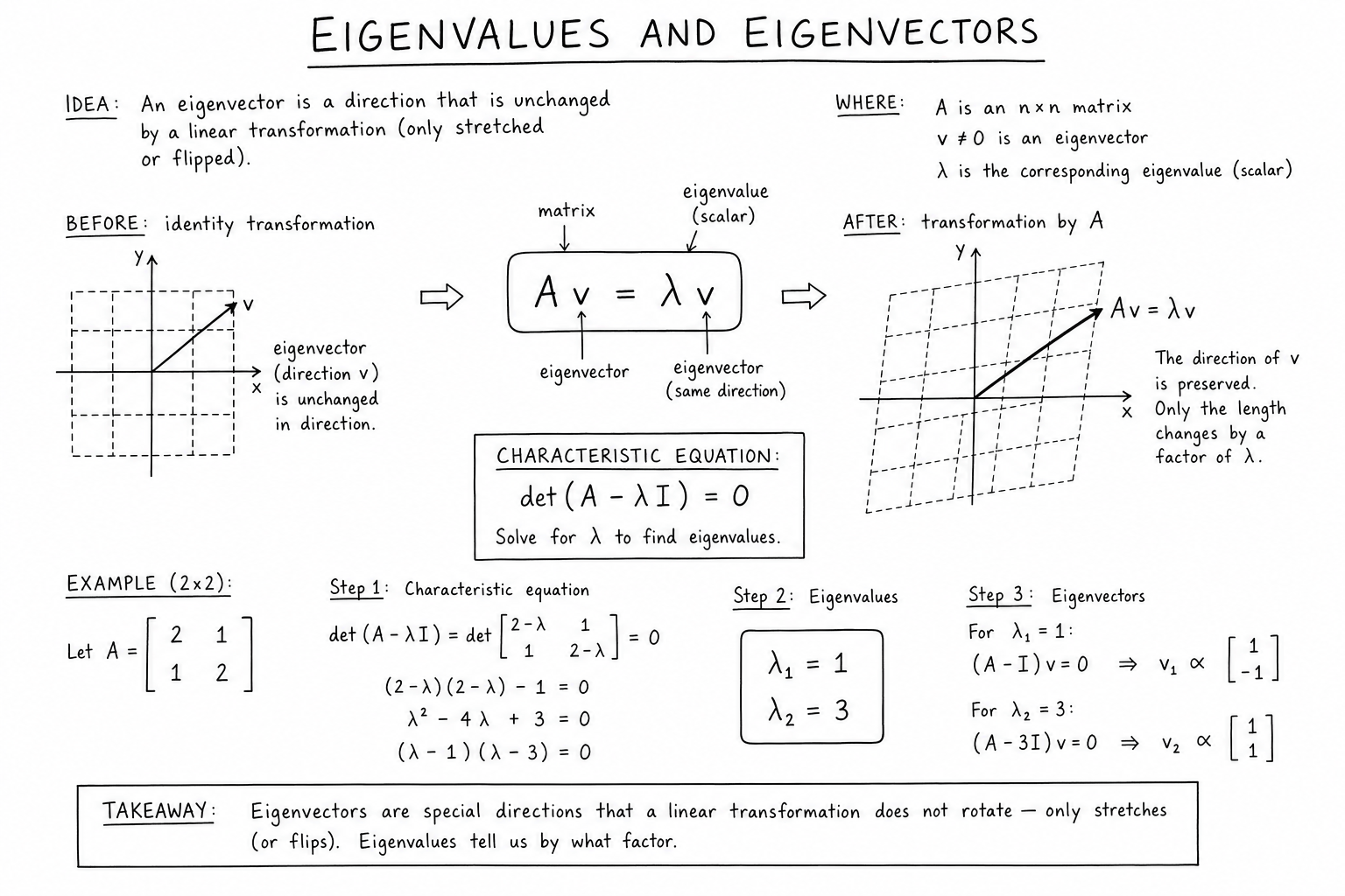
The defining equation is short — \(A\mathbf{v} = \lambda \mathbf{v}\) — but the implications are enormous. Eigenvectors are the “axes” of a matrix transformation; eigenvalues are how much the transformation stretches along each axis. Diagonalizing a matrix means rewriting it in its eigenvector basis, where its action becomes pure scaling.

This study note covers the definition, the characteristic polynomial, how to compute eigenvalues and eigenvectors by hand, the geometric interpretation, diagonalization, the spectral theorem, and applications across science, engineering, and machine learning.

The Definition

For a square matrix \(A\), a nonzero vector \(\mathbf{v}\) is an eigenvector if:

$$A\mathbf{v} = \lambda \mathbf{v}$$

for some scalar \(\lambda\), called the corresponding eigenvalue.

In words: an eigenvector is a vector whose direction the matrix preserves. The matrix may stretch or compress it, but it doesn’t rotate it. The factor by which it’s stretched is the eigenvalue.

Most vectors are not eigenvectors of a given matrix. They get rotated and stretched in arbitrary ways. Eigenvectors are the special exceptions — the directions that the transformation scales without rotating.

The Characteristic Polynomial

To find eigenvalues, rearrange \(A\mathbf{v} = \lambda \mathbf{v}\) as \((A – \lambda I)\mathbf{v} = \mathbf{0}\). For a nonzero \(\mathbf{v}\) to satisfy this, the matrix \(A – \lambda I\) must be singular:

$$\det(A – \lambda I) = 0$$

This is the characteristic equation, and the polynomial \(p(\lambda) = \det(A – \lambda I)\) is the characteristic polynomial. Its degree equals the matrix size; an \(n \times n\) matrix has a characteristic polynomial of degree \(n\) and therefore exactly \(n\) eigenvalues, counted with multiplicity (over the complex numbers).

Solving \(p(\lambda) = 0\) finds the eigenvalues. Once eigenvalues are known, plug each back into \((A – \lambda I)\mathbf{v} = \mathbf{0}\) and solve for \(\mathbf{v}\) to get the corresponding eigenvectors.

Worked Example: 2×2 Matrix

Find eigenvalues and eigenvectors of \(A = \begin{pmatrix} 4 & 1 \\ 2 & 3 \end{pmatrix}\).

Step 1: characteristic polynomial.

$$\det(A – \lambda I) = (4 – \lambda)(3 – \lambda) – 2 = \lambda^2 – 7\lambda + 10 = 0$$

Solving: \(\lambda_1 = 5\), \(\lambda_2 = 2\).

Step 2: eigenvector for \(\lambda_1 = 5\).

\((A – 5I)\mathbf{v} = \begin{pmatrix} -1 & 1 \\ 2 & -2 \end{pmatrix}\mathbf{v} = \mathbf{0}\). Both rows give \(v_1 = v_2\), so \(\mathbf{v}_1 = (1, 1)\).

Step 3: eigenvector for \(\lambda_2 = 2\).

\((A – 2I)\mathbf{v} = \begin{pmatrix} 2 & 1 \\ 2 & 1 \end{pmatrix}\mathbf{v} = \mathbf{0}\). Both rows give \(2v_1 + v_2 = 0\), so \(\mathbf{v}_2 = (1, -2)\).

Geometric Meaning

Imagine the matrix \(A\) as a transformation that takes 2D vectors to 2D vectors. Most input vectors come out pointing in different directions. But the eigenvectors come out pointing in the same direction (or directly opposite, if the eigenvalue is negative), only stretched.

For the example above, every vector along \((1, 1)\) gets scaled by 5 (and stays on that line). Every vector along \((1, -2)\) gets scaled by 2 (and stays on that line). Vectors not on these two lines get warped into combinations of the two stretches.

This decomposition is the heart of what eigenvalues and eigenvectors do: they identify the “stable directions” of a linear transformation and the scaling factor along each.

Diagonalization

If a square matrix \(A\) has \(n\) linearly independent eigenvectors, it can be written as:

$$A = P \Lambda P^{-1}$$

where the columns of \(P\) are the eigenvectors and \(\Lambda\) is the diagonal matrix of eigenvalues. \(A\) is then called diagonalizable.

Diagonalization makes many matrix computations easier. Powers: \(A^k = P \Lambda^k P^{-1}\), and \(\Lambda^k\) is just the eigenvalues raised to the power \(k\). Matrix exponentials: \(e^A = P e^\Lambda P^{-1}\). Solving differential equations \(\dot{\mathbf{x}} = A\mathbf{x}\) reduces to scalar equations along eigenvector directions.

Not every matrix is diagonalizable. Defective matrices (missing eigenvectors) require Jordan canonical form instead. In practice, many matrices are diagonalizable enough that this concern rarely matters in applied work.

The Spectral Theorem

For real symmetric matrices, the spectral theorem guarantees:

1. All eigenvalues are real.
2. Eigenvectors corresponding to distinct eigenvalues are orthogonal.
3. The matrix is diagonalizable, and there exists an orthonormal basis of eigenvectors.

So \(A = Q \Lambda Q^T\) where \(Q\) is an orthogonal matrix (columns are orthonormal eigenvectors). The transpose replaces the inverse, simplifying many computations.

The spectral theorem is one of the cleanest results in linear algebra and is the backbone of principal component analysis, spectral graph theory, and quantum mechanics. Symmetric matrices appear constantly in applied math (covariance matrices, Hessians, Laplacians), so the spectral theorem applies to nearly every applied problem.

Properties of Eigenvalues

• Trace: the sum of eigenvalues equals the trace of the matrix (sum of diagonal entries).
• Determinant: the product of eigenvalues equals the determinant.
• Inverse: if \(A\) is invertible, the eigenvalues of \(A^{-1}\) are \(1/\lambda_i\), with the same eigenvectors.
• Powers: the eigenvalues of \(A^k\) are \(\lambda_i^k\), with the same eigenvectors.
• Transpose: \(A^T\) has the same eigenvalues as \(A\) (but generally different eigenvectors).
• Polynomial: if \(p(\lambda)\) is any polynomial, the eigenvalues of \(p(A)\) are \(p(\lambda_i)\).

These properties let you compute many derived quantities (determinants, traces, condition numbers) from eigenvalues without re-doing the full matrix work.

Complex Eigenvalues

Real matrices can have complex eigenvalues. They come in conjugate pairs: if \(a + bi\) is an eigenvalue, so is \(a – bi\). Geometrically, complex eigenvalues correspond to rotational components of the transformation.

A pure rotation matrix \(\begin{pmatrix} \cos\theta & -\sin\theta \\ \sin\theta & \cos\theta \end{pmatrix}\) has eigenvalues \(e^{\pm i\theta}\). The angle \(\theta\) of rotation appears directly in the complex eigenvalues. Magnitude 1 means no scaling, only rotation.

Complex eigenvalues show up in oscillatory dynamical systems, AC circuit analysis, and the analysis of Markov chains with periodic structure. Working with them requires comfort with complex numbers but produces no new fundamental difficulties.

PCA: Eigenvalues for Data Science

Principal Component Analysis (PCA) decomposes the covariance matrix of a dataset into eigenvectors and eigenvalues. The eigenvectors give the principal directions of variance; the eigenvalues give the variance along each direction.

Project the data onto the first few eigenvectors (those with the largest eigenvalues) to get a low-dimensional representation that preserves most of the variance. This is the standard dimensionality reduction technique in data science and machine learning.

PCA is used for visualization (project to 2D for plotting), feature reduction (use top \(k\) components instead of all features), noise reduction (small eigenvalues are usually noise), and exploratory analysis. The fact that all of this works elegantly traces back to the spectral theorem applied to the symmetric covariance matrix.

PageRank: Eigenvalues for Search

Google’s original PageRank algorithm computes the principal eigenvector of the web’s link matrix. Web pages are nodes; links are weighted edges. The PageRank score of each page is the corresponding entry of the eigenvector associated with the largest eigenvalue.

The interpretation: PageRank is the long-run probability that a random surfer is at a given page. The link matrix is a Markov chain transition matrix; its dominant eigenvector is the stationary distribution. Eigenvalue analysis gave Google a principled, scalable way to rank web pages and helped launch the modern search era.

Vibration Analysis and Dynamical Systems

Engineers analyze structural vibrations by computing eigenvalues and eigenvectors of mass and stiffness matrices. Eigenvalues give the natural frequencies; eigenvectors give the corresponding mode shapes.

Bridges, buildings, aircraft, and engines all depend on knowing where these resonant frequencies sit relative to expected loads. The Tacoma Narrows bridge collapse in 1940 is the textbook cautionary tale of eigenfrequency mismatch with environmental forcing.

The same math underlies stability analysis of control systems and ordinary differential equation systems. Negative real eigenvalues mean stable equilibria; positive real eigenvalues mean instability; complex eigenvalues with negative real parts mean damped oscillations.

Quantum Mechanics

In quantum mechanics, observables are represented by Hermitian operators (the complex-matrix analogue of symmetric matrices). The possible measurement outcomes are the eigenvalues of the operator; the corresponding eigenvectors are the eigenstates.

Energy levels of an atom are eigenvalues of the Hamiltonian operator. Spin states are eigenvectors of spin operators. The entire formalism of quantum mechanics is built on eigenvalue equations like \(H\psi = E\psi\) — the Schrödinger equation in time-independent form.

Numerical Computation

Computing eigenvalues by hand is fine for 2×2 and 3×3 matrices. Beyond that, characteristic polynomials become unwieldy and high-degree polynomial roots are numerically unstable.

Modern algorithms compute eigenvalues iteratively. The QR algorithm (Francis, 1961) is the standard for general dense matrices. The Lanczos and Arnoldi methods handle large sparse matrices, computing only a few eigenvalues at a time. Power iteration is the simplest method and works well when only the largest eigenvalue is needed (PageRank uses a variant of this).

NumPy, MATLAB, and LAPACK all implement these algorithms efficiently. For most practical work, you call a library function and trust the implementation; understanding the algorithms matters when you hit numerical issues or work with structured matrices that admit faster methods.

Common Mistakes With Eigenvalues

1. Forgetting that eigenvectors are nonzero by definition. The zero vector trivially satisfies \(A\mathbf{0} = \lambda \mathbf{0}\) for any \(\lambda\), so we exclude it.
2. Treating eigenvectors as unique. Any nonzero scalar multiple of an eigenvector is also an eigenvector. The eigenvector direction is unique; the magnitude is conventional (often normalized to unit length).
3. Assuming all matrices are diagonalizable. Defective matrices have fewer eigenvectors than their dimension and require Jordan form instead.
4. Computing eigenvalues by characteristic polynomial for large matrices. The polynomial roots are numerically unstable; use iterative algorithms (QR, Lanczos) instead.
5. Forgetting that complex eigenvalues come in conjugate pairs for real matrices. If \(a + bi\) is an eigenvalue, so is \(a – bi\).
6. Confusing eigenvalues of \(A\) with eigenvalues of \(A + cI\). The latter are \(\lambda + c\), shifted by the same constant.

Why Eigenvalues Are So Useful

Eigenvalues and eigenvectors decompose a transformation into scaling factors along independent directions. Almost every “structural” question about a matrix reduces to its eigenvalue structure: stability, condition number, principal directions of variation, natural frequencies, asymptotic behavior, dimensionality reduction.

The unifying insight is this: a generic linear transformation looks complicated in arbitrary coordinates, but in the eigenvector basis it’s just diagonal — pure scaling. Diagonal matrices are trivially understood. Eigenvalue analysis is the systematic search for the coordinate system in which any transformation becomes simple.

A Brief History

Eigenvalues appeared first in mid-19th-century work on conic sections and quadratic forms. Augustin-Louis Cauchy proved the spectral theorem for symmetric matrices in 1829. David Hilbert generalized eigenvalue concepts to infinite-dimensional spaces in the early 20th century, paving the way for quantum mechanics. The terms eigenvalue and eigenvector come from the German Eigenwert and Eigenvektor (literally “own-value” and “own-vector”), introduced by David Hilbert.

The 20th century made eigenvalue computation practical. The QR algorithm (1961) enabled efficient computation for general dense matrices. Modern numerical linear algebra continues to extend the toolkit to massive sparse matrices and structured problems.

Singular Value Decomposition (SVD)

Singular Value Decomposition generalizes eigenvalue decomposition to non-square matrices. Any \(m \times n\) matrix \(A\) factors as \(A = U \Sigma V^T\), where \(U\) and \(V\) are orthogonal matrices and \(\Sigma\) is a diagonal matrix of nonnegative singular values.

SVD always exists. Its singular values reveal the matrix’s effective rank, condition number, and intrinsic structure. Truncating SVD to keep only the top \(k\) singular values gives the best rank-\(k\) approximation under several natural error norms — the basis for low-rank methods, image compression, and PCA.

SVD is one of the most useful results in applied linear algebra. It underpins recommender systems (Netflix challenge), latent semantic analysis in NLP, and the majority of dimensionality reduction techniques in machine learning.

Spectral Graph Theory and Network Analysis

The eigenvalues of a graph’s adjacency matrix or Laplacian reveal structural properties of the network. The second-smallest eigenvalue of the Laplacian (Fiedler eigenvalue) measures graph connectivity. The corresponding eigenvector partitions the graph into well-connected clusters — the foundation of spectral clustering.

Spectral methods for graph analysis power community detection in social networks, recommender system clustering, image segmentation, and many other modern data science tasks. They translate combinatorial graph problems into linear algebra problems that scale to enormous datasets via sparse eigenvalue solvers.

Power Iteration: The Simplest Eigenvalue Algorithm

Power iteration finds the dominant eigenvector of a matrix. Start with a random vector \(\mathbf{x}_0\). Repeatedly compute \(\mathbf{x}_{k+1} = A \mathbf{x}_k / \|A\mathbf{x}_k\|\). The sequence converges to the eigenvector with the largest absolute eigenvalue.

The convergence rate depends on the gap between the largest and second-largest eigenvalues. Bigger gap, faster convergence. Power iteration is simple, scales to enormous sparse matrices, and is the algorithm behind PageRank’s web-scale eigenvalue computation. More sophisticated methods (inverse iteration, Lanczos, Arnoldi) extend the same basic idea to compute multiple eigenvalues efficiently.

FAQs