Matrices

Matrices in linear algebra are rectangular arrays of numbers that encode linear transformations, systems of equations, datasets, graphs, and more. They’re the central computational object of linear algebra and the workhorse of nearly every algorithm in data science, machine learning, computer graphics, and engineering.

A matrix is two things at once. Computationally, it’s a grid of numbers you can add, multiply, and invert. Conceptually, it’s a linear function — a rule that takes vectors as input and produces vectors as output. Holding both views simultaneously is the mental shift that turns matrix algebra from rote calculation into structural thinking.

This study note covers matrix notation, addition and scalar multiplication, matrix multiplication and its non-commutativity, the identity and inverse matrices, the transpose, determinants and their geometric meaning, the connection to systems of linear equations, applications, and common pitfalls.

Notation and Dimensions

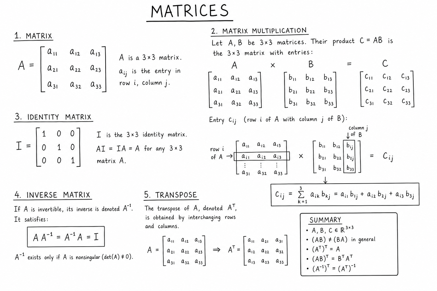
A matrix is denoted with a capital letter and its entries with subscripts: \(A_{ij}\) is the entry in row \(i\), column \(j\). An \(m \times n\) matrix has \(m\) rows and \(n\) columns:

$$A = \begin{pmatrix} a_{11} & a_{12} & \cdots & a_{1n} \\ a_{21} & a_{22} & \cdots & a_{2n} \\ \vdots & \vdots & \ddots & \vdots \\ a_{m1} & a_{m2} & \cdots & a_{mn} \end{pmatrix}$$

Square matrices have \(m = n\). Row vectors are \(1 \times n\); column vectors are \(m \times 1\). The dimensions matter for every operation — addition requires identical dimensions; multiplication requires the inner dimensions to match.

Matrix Addition and Scalar Multiplication

Matrices of the same dimension add entry-wise:

$$(A + B)_{ij} = A_{ij} + B_{ij}$$

Scalar multiplication scales every entry:

$$(cA)_{ij} = c \cdot A_{ij}$$

Both operations are commutative and associative. The zero matrix (all entries zero) is the additive identity. Together with these operations, the set of \(m \times n\) matrices forms a vector space.

Matrix Multiplication

Matrix multiplication is the most important matrix operation. To multiply \(A\) (\(m \times n\)) by \(B\) (\(n \times p\)), the product \(AB\) is an \(m \times p\) matrix with entries:

$$(AB)_{ij} = \sum_{k=1}^{n} A_{ik} B_{kj}$$

Row \(i\) of \(A\) dotted with column \(j\) of \(B\) gives entry \((i, j)\) of \(AB\). The inner dimensions must match (the number of columns of \(A\) equals the number of rows of \(B\)); the outer dimensions become the dimensions of the product.

Matrix multiplication is associative: \((AB)C = A(BC)\). It’s distributive over addition: \(A(B + C) = AB + AC\). It is not commutative: in general, \(AB \neq BA\). This non-commutativity is the source of much of linear algebra’s depth and most of its initial confusion for beginners.

Why Matrix Multiplication Is Defined That Way

The “row times column” rule looks arbitrary but encodes function composition. Each matrix represents a linear transformation. The product \(AB\) represents the composition: first apply \(B\), then apply \(A\). The strange-looking formula is exactly what makes \((AB)\mathbf{x} = A(B\mathbf{x})\) hold for all input vectors \(\mathbf{x}\).

This is also why the order matters. Composing transformations in the order “first \(B\), then \(A\)” generally produces a different result from “first \(A\), then \(B\).” Even commuting transformations (rotations about a fixed axis, scalings) don’t generalize: arbitrary linear maps don’t commute. This non-commutativity is what makes linear algebra interesting.

The Identity Matrix

The identity matrix \(I_n\) is the \(n \times n\) square matrix with 1s on the diagonal and 0s elsewhere:

$$I_3 = \begin{pmatrix} 1 & 0 & 0 \\ 0 & 1 & 0 \\ 0 & 0 & 1 \end{pmatrix}$$

The identity satisfies \(IA = AI = A\) for any compatible matrix \(A\). It’s the multiplicative identity for square matrices. Geometrically, the identity matrix represents the “do nothing” linear transformation: it leaves every vector unchanged.

The identity matrix appears constantly in proofs, inverse calculations, and matrix decompositions. It’s also the natural starting point for many iterative algorithms (start with the identity and modify from there).

The Inverse Matrix

For a square matrix \(A\), the inverse \(A^{-1}\) is the matrix satisfying \(AA^{-1} = A^{-1}A = I\). Not every square matrix has an inverse — those that do are called invertible or nonsingular; those that don’t are singular.

For a 2×2 matrix:

$$A^{-1} = \frac{1}{\det A} \begin{pmatrix} d & -b \\ -c & a \end{pmatrix} \text{ where } A = \begin{pmatrix} a & b \\ c & d \end{pmatrix}$$

For larger matrices, computing the inverse uses Gauss-Jordan elimination, LU decomposition, or other numerical algorithms. Inverses solve the matrix equation \(A\mathbf{x} = \mathbf{b}\): \(\mathbf{x} = A^{-1}\mathbf{b}\) — but in practice, never compute the inverse explicitly when you can solve the system directly via elimination, which is faster and more numerically stable.

The Transpose

The transpose \(A^T\) swaps rows and columns: \((A^T)_{ij} = A_{ji}\). An \(m \times n\) matrix becomes \(n \times m\) when transposed.

Properties: \((A^T)^T = A\), \((A + B)^T = A^T + B^T\), \((AB)^T = B^T A^T\) (note the order reversal), \((cA)^T = c A^T\).

A matrix is symmetric if \(A^T = A\); it’s skew-symmetric if \(A^T = -A\). Symmetric matrices are central to many applications: covariance matrices in statistics, Hessian matrices in optimization, adjacency matrices of undirected graphs, stiffness matrices in finite element analysis. Symmetric matrices have especially clean spectral properties — all eigenvalues are real and orthonormal eigenvector bases always exist.

Determinants

The determinant \(\det(A)\) of a square matrix is a scalar that measures how the matrix scales volumes (or signed volumes). For a 2×2 matrix:

$$\det \begin{pmatrix} a & b \\ c & d \end{pmatrix} = ad – bc$$

Geometrically, this equals the signed area of the parallelogram with sides given by the matrix’s column vectors. In 3D, the determinant equals the signed volume of the parallelepiped spanned by the columns.

Key properties: \(\det(AB) = \det(A)\det(B)\), \(\det(A^T) = \det(A)\), \(\det(A^{-1}) = 1/\det(A)\). The matrix is invertible if and only if its determinant is nonzero. A determinant of zero means the matrix collapses some volume to zero — it has linearly dependent columns and is therefore singular.

Systems of Linear Equations

The matrix equation \(A\mathbf{x} = \mathbf{b}\) represents a system of linear equations. The matrix \(A\) holds the coefficients; the vector \(\mathbf{x}\) holds the unknowns; \(\mathbf{b}\) holds the right-hand-side constants.

Three possibilities:

1. Unique solution: \(A\) is invertible (square and nonsingular). Then \(\mathbf{x} = A^{-1}\mathbf{b}\), or compute via Gauss-Jordan elimination.
2. No solution: the system is inconsistent (the vector \(\mathbf{b}\) is not in the column space of \(A\)).
3. Infinitely many solutions: the system is consistent but underdetermined; the solution set is a flat affine subspace.

This trichotomy is the foundation of solving linear systems and underpins regression, optimization, and most of numerical linear algebra.

Special Types of Matrices

• Diagonal: nonzero entries only on the main diagonal. Easy to multiply, invert, and exponentiate.
• Triangular: upper or lower triangular. Solving systems with triangular matrices is fast (forward or back substitution) — the basis for LU decomposition.
• Symmetric: \(A^T = A\). Real eigenvalues, orthonormal eigenvectors. Central in statistics and optimization.
• Orthogonal: \(Q^T Q = I\). Preserves lengths and angles. Rotations and reflections are orthogonal matrices.
• Sparse: mostly zero entries. Storage and computation use special algorithms; central in scientific computing and machine learning at scale.
• Identity, Zero, Permutation, Hermitian (complex symmetric), Unitary (complex orthogonal), Positive definite — each carries useful structure for specific applications.

Matrix Decompositions

Many matrix algorithms work by decomposing a matrix into simpler factors. Common decompositions:

• LU: \(A = LU\) where \(L\) is lower triangular and \(U\) is upper triangular. Used for solving linear systems efficiently.
• QR: \(A = QR\) where \(Q\) is orthogonal and \(R\) is upper triangular. Used for least-squares regression.
• Cholesky: \(A = LL^T\) for symmetric positive-definite matrices. Faster than LU for these matrices.
• Eigendecomposition: \(A = V \Lambda V^{-1}\) where columns of \(V\) are eigenvectors and \(\Lambda\) is diagonal of eigenvalues.
• Singular Value Decomposition (SVD): \(A = U \Sigma V^T\), the most general decomposition; underpins PCA, low-rank approximation, and recommender systems.

Decompositions reveal structure and enable efficient algorithms. Modern numerical linear algebra is largely the engineering of robust decomposition algorithms for huge matrices.

Worked Example: Matrix Multiplication

Multiply \(A = \begin{pmatrix} 1 & 2 \\ 3 & 4 \end{pmatrix}\) and \(B = \begin{pmatrix} 5 & 6 \\ 7 & 8 \end{pmatrix}\):

$$AB = \begin{pmatrix} 1 \cdot 5 + 2 \cdot 7 & 1 \cdot 6 + 2 \cdot 8 \\ 3 \cdot 5 + 4 \cdot 7 & 3 \cdot 6 + 4 \cdot 8 \end{pmatrix} = \begin{pmatrix} 19 & 22 \\ 43 & 50 \end{pmatrix}$$

Now \(BA\):

$$BA = \begin{pmatrix} 5 \cdot 1 + 6 \cdot 3 & 5 \cdot 2 + 6 \cdot 4 \\ 7 \cdot 1 + 8 \cdot 3 & 7 \cdot 2 + 8 \cdot 4 \end{pmatrix} = \begin{pmatrix} 23 & 34 \\ 31 & 46 \end{pmatrix}$$

\(AB \neq BA\). The non-commutativity is concrete: same matrices, different order, completely different products.

Where Matrices Show Up in Practice

• Machine learning: data is stored as matrices (rows = examples, columns = features). Neural network weights are matrices. Convolution operations multiply matrices behind the scenes. Read more in best machine learning courses.
• Computer graphics: 3D transformations (translation, rotation, scaling) are 4×4 matrix operations applied to homogeneous coordinates.
• Statistics: covariance matrices, regression coefficient matrices, correlation matrices, Hat matrices in linear regression.
• Engineering: stiffness matrices in finite element analysis, transfer matrices in control systems, scattering matrices in optics and electromagnetics.
• Network analysis: adjacency matrices of graphs, Laplacian matrices for spectral methods, transition matrices for Markov chains.
• Quantum mechanics: state vectors transformed by unitary matrices; observables represented by Hermitian matrices.

Common Mistakes With Matrices

1. Assuming \(AB = BA\). Matrix multiplication is generally not commutative. Always preserve order.
2. Mismatched dimensions. The product \(AB\) requires the number of columns of \(A\) to equal the number of rows of \(B\). Software gives explicit errors; mental computation often skips this check.
3. Computing the inverse when you don’t need to. Solving \(A\mathbf{x} = \mathbf{b}\) by computing \(A^{-1}\) and multiplying is slower and less stable than direct elimination.
4. Confusing inverse with transpose. \(A^T\) and \(A^{-1}\) are different operations. They coincide only for orthogonal matrices.
5. Treating singular matrices as if they were invertible. A determinant of zero means no inverse exists. Always check determinant or rank before assuming invertibility.

A Brief History of Matrices

The Chinese mathematical text The Nine Chapters on the Mathematical Art (~200 BCE) describes solving systems of linear equations using array manipulations equivalent to Gaussian elimination — over two thousand years before the West formalized the technique.

The term “matrix” was coined by James Joseph Sylvester in 1850. Arthur Cayley developed matrix algebra in the 1850s and 1860s, including matrix multiplication, the inverse, and the characteristic polynomial. By the early 20th century, matrices had become central to physics (quantum mechanics is matrix mechanics) and engineering.

The modern era of matrix algorithms began with John von Neumann and Herman Goldstine in the 1940s as they developed numerical methods for early computers. LAPACK (Linear Algebra PACKage), released in 1992 and still maintained, is the canonical reference implementation for dense matrix algorithms and underpins NumPy, MATLAB, R, Julia, and most scientific computing software in use today.

Matrix Conditioning and Numerical Stability

The condition number of a matrix measures how sensitive its solutions are to perturbations in the input. A well-conditioned matrix produces stable solutions; an ill-conditioned matrix amplifies tiny input errors into huge output errors.

Formally, the condition number is \(\kappa(A) = \|A\| \cdot \|A^{-1}\|\). Large condition numbers (above \(10^6\) or so) signal numerical trouble. Solutions to ill-conditioned systems may be wildly wrong even with small floating-point errors.

Diagnosing and remedying ill-conditioning is a daily concern in scientific computing, machine learning (poorly scaled features create ill-conditioned design matrices), and engineering simulation. Regularization, preconditioning, and feature scaling all address this.

Sparse Matrices and Their Algorithms

A sparse matrix has mostly zero entries. Storing only the nonzero entries (and their positions) saves enormous memory. Algorithms designed for sparse matrices skip the zero entries entirely, achieving massive speedups for the same problem.

Compressed sparse row (CSR) and compressed sparse column (CSC) are the standard storage formats. Iterative solvers (conjugate gradient, GMRES) and sparse factorization methods (sparse LU, sparse Cholesky) handle large sparse systems that would be impossible to solve with dense algorithms.

Sparse matrices appear constantly in finite element analysis, large-scale optimization, web graphs (PageRank’s link matrix is sparse), and recommender systems (user-item matrices are mostly empty). Modern scientific computing leans heavily on sparse linear algebra.

Tensors as Generalizations of Matrices

Tensors generalize matrices to multi-index arrays. A scalar is a rank-0 tensor; a vector is rank-1; a matrix is rank-2; a 3D array of numbers is rank-3; and so on. Tensors are the natural data structure for physical quantities (stress, strain, electromagnetic field), multi-dimensional signal processing, and modern deep learning (input batches are 4D tensors: batch × channels × height × width).

Tensor operations generalize matrix operations. Tensor contraction generalizes matrix multiplication. Einstein notation provides a compact way to express complex tensor operations. PyTorch, TensorFlow, and JAX are essentially tensor manipulation libraries; the “matrix” in matrix algorithms is just a convenient 2D special case of the underlying tensor framework.

Block Matrices and Block Operations

Large matrices can be partitioned into blocks (sub-matrices), and many operations work block-wise. Block multiplication mirrors scalar multiplication: \(\begin{pmatrix} A & B \\ C & D \end{pmatrix} \begin{pmatrix} E & F \\ G & H \end{pmatrix} = \begin{pmatrix} AE + BG & AF + BH \\ CE + DG & CF + DH \end{pmatrix}\) when block dimensions match.

Block matrices appear constantly in numerical algorithms. Schur complements decompose block-structured matrices into smaller solves. Strassen’s algorithm uses block matrix tricks to multiply matrices faster than the naive \(O(n^3)\) bound. Modern dense matrix libraries (BLAS Level 3) work primarily on blocks rather than individual entries.

FAQs