Vectors

Vectors in linear algebra are quantities with both magnitude and direction. They’re the foundational object of nearly every quantitative field — physics describes forces and velocities as vectors, computer graphics encodes positions and lighting as vectors, machine learning models represent data points and gradients as vectors. Once you understand vectors, you have the basic vocabulary for most of applied mathematics.

The trick is to hold two views simultaneously. Geometrically, a vector is an arrow with length and direction. Algebraically, a vector is a tuple of numbers (the components). Both views are correct, both are useful, and most insights come from translating between them. Operations on vectors look one way as arrow manipulations and another way as arithmetic on components — and the two views always agree.

This study note covers the geometric and algebraic definitions, the standard operations (addition, scalar multiplication, dot product, cross product), magnitudes and unit vectors, projections, linear independence, the geometric meaning of all the operations, and applications across science, engineering, and machine learning.

The Two Views of a Vector

Geometrically, a vector is an arrow in space with a specific length (magnitude) and direction, but no fixed location. Two arrows with the same length and direction are the same vector, regardless of where they’re drawn.

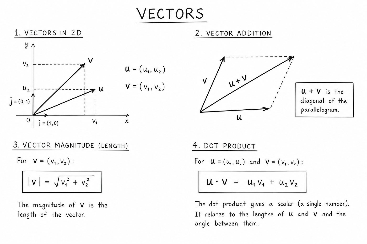
Algebraically, a vector is an ordered tuple of numbers — its components. A 2D vector is \((v_1, v_2)\); a 3D vector is \((v_1, v_2, v_3)\); an \(n\)-dimensional vector is \((v_1, v_2, \ldots, v_n)\). Each component represents the projection of the vector onto a coordinate axis.

The two views are equivalent. The arrow from the origin to the point \((3, 4)\) is the same vector as the algebraic object \((3, 4)\). Most linear algebra builds on switching freely between these representations.

Components in a Coordinate System

Choose a coordinate system (axes), and a vector decomposes into components along each axis. In 2D with standard axes:

$$\mathbf{v} = (v_1, v_2) = v_1 \hat{i} + v_2 \hat{j}$$

where \(\hat{i} = (1, 0)\) and \(\hat{j} = (0, 1)\) are unit vectors along the x and y axes.

In 3D, add \(\hat{k} = (0, 0, 1)\):

$$\mathbf{v} = v_1 \hat{i} + v_2 \hat{j} + v_3 \hat{k}$$

Components depend on the coordinate system. The same geometric arrow has different components in different bases — a key insight that motivates change-of-basis transformations and the entire theory of linear transformations.

Vector Addition

To add two vectors algebraically, add their components:

$$\mathbf{u} + \mathbf{v} = (u_1 + v_1, u_2 + v_2, \ldots)$$

Geometrically, place the tail of \(\mathbf{v}\) at the head of \(\mathbf{u}\); the sum is the arrow from the tail of \(\mathbf{u}\) to the head of \(\mathbf{v}\). This is the triangle rule (or parallelogram rule, when the two vectors share a tail and you complete the parallelogram).

Vector addition is commutative and associative: \(\mathbf{u} + \mathbf{v} = \mathbf{v} + \mathbf{u}\) and \((\mathbf{u} + \mathbf{v}) + \mathbf{w} = \mathbf{u} + (\mathbf{v} + \mathbf{w})\). The zero vector \(\mathbf{0}\) is the additive identity. Every vector \(\mathbf{v}\) has an additive inverse \(-\mathbf{v}\) with the same length but opposite direction.

Scalar Multiplication

Multiplying a vector by a scalar (a real number) scales each component:

$$c \mathbf{v} = (c v_1, c v_2, \ldots)$$

Geometrically, scalar multiplication stretches or compresses the vector. Multiplying by a positive scalar keeps the direction; multiplying by a negative scalar reverses it. Multiplying by zero collapses the vector to the zero vector.

Scalar multiplication distributes over vector addition: \(c(\mathbf{u} + \mathbf{v}) = c\mathbf{u} + c\mathbf{v}\). It also satisfies \((cd)\mathbf{v} = c(d\mathbf{v})\) and \(1 \cdot \mathbf{v} = \mathbf{v}\). These properties, plus the addition properties, make the set of vectors a vector space.

Magnitude and Unit Vectors

The magnitude (length, norm) of a vector is computed by the Pythagorean theorem extended to \(n\) dimensions:

$$|\mathbf{v}| = \sqrt{v_1^2 + v_2^2 + \ldots + v_n^2}$$

A unit vector has magnitude 1. To turn any nonzero vector into a unit vector pointing in the same direction, divide by its magnitude:

$$\hat{v} = \frac{\mathbf{v}}{|\mathbf{v}|}$$

Unit vectors are useful when only the direction matters — defining axes, expressing other vectors as scalar multiples, or computing angles. The standard basis vectors \(\hat{i}\), \(\hat{j}\), \(\hat{k}\) are the canonical example.

The Dot Product

The dot product (also called inner product or scalar product) of two vectors is defined two equivalent ways:

$$\mathbf{u} \cdot \mathbf{v} = u_1 v_1 + u_2 v_2 + \ldots + u_n v_n = |\mathbf{u}||\mathbf{v}| \cos\theta$$

where \(\theta\) is the angle between the vectors. The first form is computational (just multiply components and add); the second form is geometric (and shows the dot product encodes the angle).

Key consequence: if \(\mathbf{u} \cdot \mathbf{v} = 0\) and neither vector is zero, the vectors are perpendicular (orthogonal). The dot product is the standard test for orthogonality, and orthogonality is one of the most useful structural properties in all of linear algebra.

The Cross Product (3D Only)

In 3D, the cross product produces a vector perpendicular to both inputs:

$$\mathbf{u} \times \mathbf{v} = (u_2 v_3 – u_3 v_2, u_3 v_1 – u_1 v_3, u_1 v_2 – u_2 v_1)$$

The magnitude equals \(|\mathbf{u}||\mathbf{v}| \sin\theta\), the area of the parallelogram spanned by the two vectors. Direction follows the right-hand rule.

The cross product is anticommutative: \(\mathbf{u} \times \mathbf{v} = -(\mathbf{v} \times \mathbf{u})\). It only exists in 3D and 7D — there’s no consistent way to define a perpendicular-vector product in other dimensions. In physics, torque, angular momentum, and magnetic force all use cross products.

Projections

The projection of \(\mathbf{u}\) onto \(\mathbf{v}\) is the component of \(\mathbf{u}\) along the direction of \(\mathbf{v}\):

$$\text{proj}_{\mathbf{v}} \mathbf{u} = \frac{\mathbf{u} \cdot \mathbf{v}}{|\mathbf{v}|^2} \mathbf{v}$$

Geometrically, drop a perpendicular from the head of \(\mathbf{u}\) onto the line containing \(\mathbf{v}\); the projection is the vector along \(\mathbf{v}\) from origin to the foot of the perpendicular.

Projections decompose vectors into parallel and perpendicular components: \(\mathbf{u} = \text{proj}_{\mathbf{v}} \mathbf{u} + (\mathbf{u} – \text{proj}_{\mathbf{v}} \mathbf{u})\). The perpendicular piece is the residual after removing the parallel component. Projections underlie least-squares regression, Gram-Schmidt orthogonalization, and most decomposition methods in linear algebra.

Linear Combinations and Span

A linear combination of vectors \(\mathbf{v}_1, \mathbf{v}_2, \ldots, \mathbf{v}_k\) is any expression of the form \(c_1 \mathbf{v}_1 + c_2 \mathbf{v}_2 + \ldots + c_k \mathbf{v}_k\) where the \(c_i\) are scalars.

The set of all linear combinations is the span of those vectors. In 2D, the span of two non-parallel vectors is the entire plane. In 3D, the span of three non-coplanar vectors is all of \(\mathbb{R}^3\).

Span is the basic notion of “what can I build from these vectors using addition and scaling?” It leads to the ideas of basis (a minimal spanning set), dimension (the size of any basis), and rank (the dimension of the column span of a matrix). Read more in discrete math books for computer science.

Linear Independence

A set of vectors is linearly independent if no vector in the set can be written as a linear combination of the others. Equivalently, the only way to get \(c_1 \mathbf{v}_1 + c_2 \mathbf{v}_2 + \ldots + c_k \mathbf{v}_k = \mathbf{0}\) is by setting all \(c_i = 0\).

Linear independence is what guarantees a set of vectors carries non-redundant information. In 3D, three linearly independent vectors form a basis: every other vector can be written uniquely as a combination of them. Adding a fourth vector to that set must produce linear dependence.

Linear independence is computationally tested by row-reducing a matrix whose columns are the vectors and checking the rank. Software libraries (NumPy, MATLAB, R) handle this routinely; understanding the structure matters for diagnosing problems in regression (multicollinearity), graphics (degenerate triangle meshes), and dynamics (degenerate constraints).

Vector Spaces

A vector space is a set of objects (called vectors) closed under addition and scalar multiplication, satisfying eight axioms (associativity, commutativity, identities, inverses, distributivity, etc.). The familiar \(\mathbb{R}^n\) is the canonical vector space, but the concept generalizes to function spaces, polynomial spaces, matrices, and even more abstract structures.

Subspaces are subsets that are themselves vector spaces — closed under the operations of the parent space. The span of any set of vectors is automatically a subspace. Solutions to homogeneous linear systems form subspaces. Eigenspaces (the span of all eigenvectors for a given eigenvalue) are subspaces.

The abstraction matters because results proven for general vector spaces apply to all the special cases: \(n\)-tuples, polynomials of degree at most \(n\), continuous functions, square-integrable functions in physics, and so on.

Worked Example: Computing Vector Quantities

Given \(\mathbf{u} = (3, 4)\) and \(\mathbf{v} = (1, 2)\):

• Sum: \(\mathbf{u} + \mathbf{v} = (4, 6)\)
• Scalar multiple: \(2 \mathbf{u} = (6, 8)\)
• Magnitude: \(|\mathbf{u}| = \sqrt{9 + 16} = 5\)
• Unit vector: \(\hat{u} = (3/5, 4/5)\)
• Dot product: \(\mathbf{u} \cdot \mathbf{v} = 3 + 8 = 11\)
• Angle: \(\cos\theta = 11 / (5 \cdot \sqrt{5}) \approx 0.984\), so \(\theta \approx 10.3°\)
• Projection of \(\mathbf{u}\) onto \(\mathbf{v}\): \(\frac{11}{5} \cdot (1, 2) / \sqrt{5} = (11/5)(1/\sqrt{5})(1,2)\)

Routine arithmetic, all from the formulas. Once these become automatic, vector calculations stop feeling like work and start feeling like sentence-level reading.

Where Vectors Show Up

• Physics: velocity, acceleration, force, momentum, electric and magnetic fields. Almost every physical quantity that has direction is a vector.
• Computer graphics: positions, normals, light directions, surface tangents. The math of 3D rendering is largely vector and matrix arithmetic.
• Machine learning: data points are vectors in feature space; gradients are vectors in parameter space; embeddings (word2vec, sentence transformers) represent semantic content as vectors.
• Robotics: joint angles, end-effector positions, control inputs. Robot kinematics is vector and matrix algebra.
• Engineering: stress and strain tensors decompose to vectors; signal processing represents signals as high-dimensional vectors.
• Geographic information systems: directions, displacements, and flow fields encoded as vectors over a spatial domain.

Vectors vs Scalars

Scalars are pure numbers — temperature, mass, energy. They have magnitude but no direction. Vectors have both. The distinction matters because operations differ: scalars combine through ordinary arithmetic; vectors require component-wise rules and direction-aware combinations.

Some quantities sit between: tensors generalize vectors to multi-index arrays (rank-2 tensors include matrices, stress tensors, electromagnetic field tensors). Spinors encode rotational properties beyond what vectors capture. The vector / tensor distinction is essential in physics and differential geometry.

For most everyday work in engineering, machine learning, and applied math, the vector vs scalar distinction is enough. Higher-rank tensors mostly appear in physics, general relativity, and certain advanced ML architectures.

Vectors in Higher Dimensions

Linear algebra extends seamlessly to dimensions far beyond the 3D physical world. Machine learning routinely uses 100-, 1000-, or million-dimensional vectors. Each dimension might represent a different feature (in tabular data), a pixel (in image data), or a component of a learned embedding (in language models).

The geometry generalizes — magnitudes, dot products, projections, and angles all work in any number of dimensions. Visualization becomes impossible past 3D, but the algebra is unchanged. Modern data science is largely the practice of treating high-dimensional vector spaces as if they had the geometric properties we know from low dimensions, then debugging when intuition breaks down (the curse of dimensionality, concentration of measure, and other high-dim surprises).

Common Mistakes With Vectors

1. Confusing position and direction. A vector has direction and magnitude but no fixed location. Position vectors specify locations only by reference to a chosen origin.
2. Forgetting that vector addition uses the parallelogram rule. You can’t just “add lengths” of two vectors unless they’re parallel.
3. Mixing up dot product and cross product. Dot product produces a scalar; cross product produces a vector. They have different geometric meanings.
4. Treating non-perpendicular vectors as if they were. Dot products and projections behave differently when vectors aren’t orthogonal — many shortcut formulas implicitly assume orthogonality.
5. Ignoring units. A vector with units (meters, newtons, m/s) cannot be added to a vector with different units. Dimensional consistency matters.
6. Mistaking a vector for its components. The same vector has different components in different coordinate systems. The components alone aren’t the vector — the components together with the chosen basis are.

A Brief History of Vectors

The modern concept of a vector emerged in the 19th century. William Rowan Hamilton developed quaternions in 1843, and Hermann Grassmann independently developed the algebra of vectors in his 1844 Ausdehnungslehre. Josiah Willard Gibbs and Oliver Heaviside later distilled vector calculus into the form taught today, removing the cumbersome quaternion notation.

Maxwell’s equations in vector form (Heaviside, 1884) revolutionized physics by replacing 20 scalar equations with 4 elegant vector equations. The 20th century extended vectors to functional analysis (Hilbert spaces, Banach spaces) and modern theoretical physics. Today, vectors are taught in undergraduate calculus, computer graphics, and data science as foundational vocabulary.

Vectors in Polar and Spherical Coordinates

Vectors don’t have to be expressed in Cartesian components. Polar coordinates use magnitude and angle: \(\mathbf{v} = (r, \theta)\). Spherical coordinates in 3D use \((\rho, \theta, \phi)\). Cylindrical coordinates use \((r, \theta, z)\).

Coordinate transformations between systems use trigonometric formulas: \(x = r\cos\theta\), \(y = r\sin\theta\). Each coordinate system has trade-offs — Cartesian is best for general work; polar simplifies rotations; spherical is natural for problems with central symmetry.

Choosing the right coordinate system can collapse a hard problem into an easy one. Quantum mechanics on a hydrogen atom uses spherical coordinates because the Coulomb potential is centrally symmetric. Fluid mechanics around a cylinder uses cylindrical coordinates. Knowing when to switch is part of the practical art of physics and engineering.

FAQs