Big-O Notation

Big-O notation describes how the resource requirements of an algorithm — usually time or space — scale with the size of the input. It’s the universal language for talking about algorithm efficiency. Whether you’re choosing between sorting algorithms, estimating database query cost, or evaluating whether your code can handle production-scale data, you’re reasoning in Big-O terms.

The notation strips away constant factors and lower-order terms, focusing on how an algorithm scales asymptotically. \(O(n^2)\) means quadratic growth: doubling the input quadruples the work. \(O(n \log n)\) means slightly worse than linear. \(O(2^n)\) means brute-force exponential blowup that becomes intractable past a few dozen items. Knowing where each common algorithm sits on this scale is half of algorithm selection.

This study note covers the formal definition, common complexity classes with examples, the difference between Big-O, Big-Theta, and Big-Omega, time vs space complexity, common mistakes, and the broader context that makes asymptotic analysis essential for working programmers.

The Formal Definition

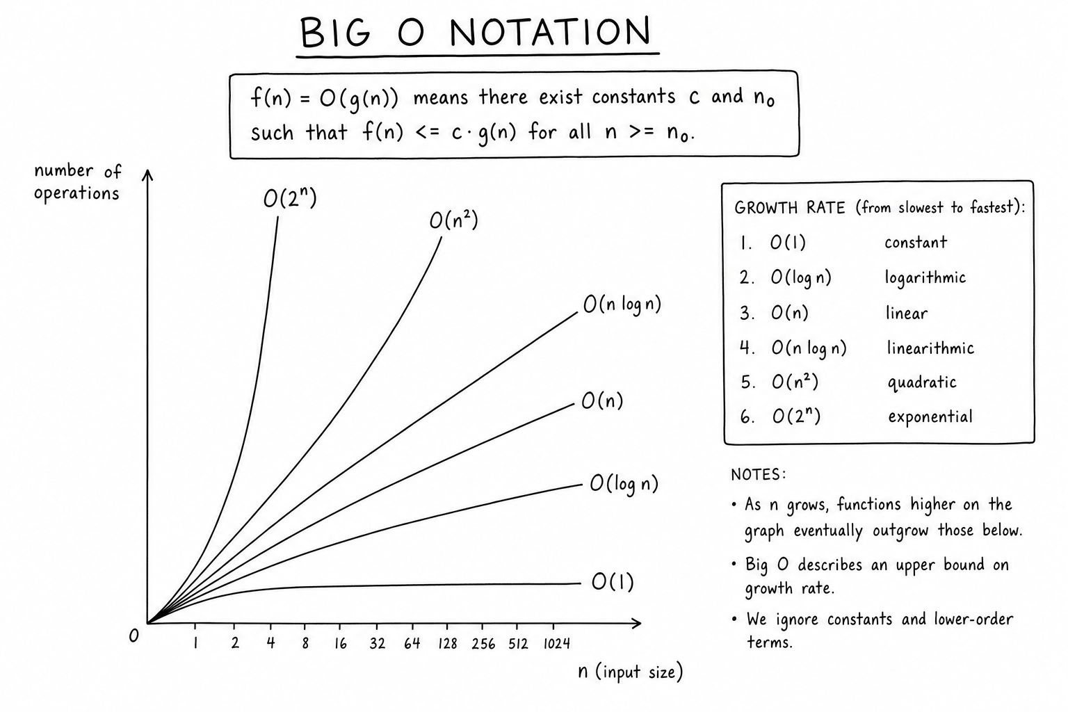
\(f(n) = O(g(n))\) means there exist positive constants \(c\) and \(n_0\) such that:

$$f(n) \leq c \cdot g(n) \quad \text{for all } n \geq n_0$$

In words: \(f(n)\) grows no faster than \(g(n)\) up to a constant factor, for all sufficiently large \(n\). This is an upper bound on growth rate. Constants and lower-order terms drop out because they become negligible as \(n\) grows.

Big-O is purely about asymptotic behavior. \(3n^2 + 100n + 9999 = O(n^2)\) — the constant 9999 and the linear term 100n become tiny compared to \(3n^2\) once \(n\) is large enough. The 3 also drops because constants don’t matter in Big-O.

Common Complexity Classes

From fastest to slowest:

• \(O(1)\) — constant. Hash table lookup, array index access. The runtime doesn’t depend on input size.
• \(O(\log n)\) — logarithmic. Binary search, balanced BST operations. Doubling the input adds only one step.
• \(O(n)\) — linear. Single-pass loops, linear search. Time scales proportionally with input size.
• \(O(n \log n)\) — linearithmic. Merge sort, heapsort, quicksort (average case). The provably optimal class for comparison-based sorting.
• \(O(n^2)\) — quadratic. Bubble sort, naive pair comparisons. Doubling input quadruples work.
• \(O(n^3)\) — cubic. Naive matrix multiplication, Floyd-Warshall. Doubling input multiplies work by 8.
• \(O(2^n)\) — exponential. Brute-force subset search, naive recursive Fibonacci. Becomes intractable past \(n \approx 30\).
• \(O(n!)\) — factorial. Brute-force traveling salesman, all permutations. Intractable past \(n \approx 12\).

Worked Example: Linear vs Quadratic

Consider two ways to find duplicates in a list of \(n\) items.

Naive (quadratic): compare every pair. \(\binom{n}{2} \approx n^2/2\) comparisons. \(O(n^2)\).

for i in range(n):
    for j in range(i+1, n):
        if items[i] == items[j]: return True

Hash-based (linear): insert each item into a set; if it’s already there, you’ve found a duplicate. \(n\) insertions, each \(O(1)\) on average. \(O(n)\).

seen = set()
for x in items:
    if x in seen: return True
    seen.add(x)

For \(n = 10{,}000\), the quadratic version does ~50 million comparisons. The linear version does ~10,000 set operations. Same problem, different complexity class, drastically different runtime. This is the kind of choice Big-O analysis informs.

Big-O vs Big-Theta vs Big-Omega

Three asymptotic notations get used together:

• \(O(g(n))\) — upper bound. Function grows no faster than \(g(n)\).
• \(\Omega(g(n))\) — lower bound. Function grows at least as fast as \(g(n)\).
• \(\Theta(g(n))\) — tight bound. Function grows exactly at the rate of \(g(n)\) (both upper and lower bound match).

In practice, programmers say “Big-O” to mean tight bound (\(\Theta\)) most of the time, even though that’s technically imprecise. When precision matters (e.g., proving lower bounds for sorting), use \(\Omega\) and \(\Theta\) explicitly.

Plotting the Complexity Classes

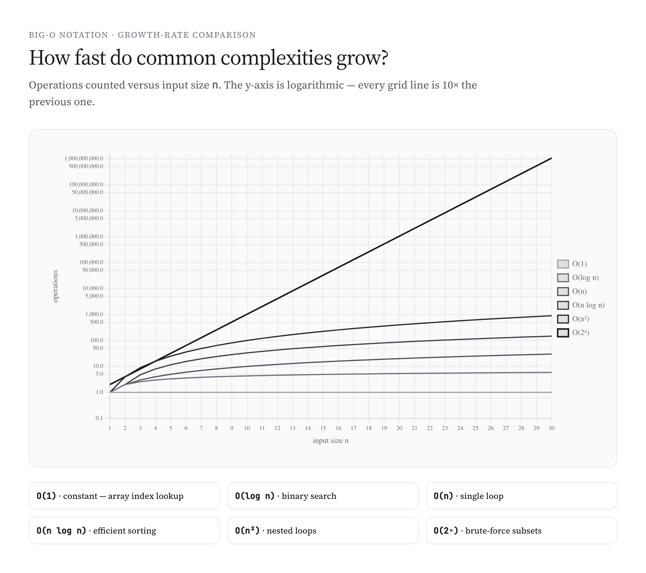
Different complexity classes look almost identical for small inputs but diverge dramatically as input grows. On a logarithmic y-axis, the differences become clear: each class shows up as a line with a distinct slope. Linear and constant complexities sit at the bottom; exponential and factorial blow up off the top.

The implication: for small inputs (\(n < 100\)), almost any algorithm works. For medium inputs (\(n < 10^6\)), \(O(n \log n)\) becomes essential. For large inputs (\(n > 10^9\)), even \(O(n)\) might be too slow, and you need sublinear or distributed algorithms.

Time Complexity vs Space Complexity

Big-O describes both time and space requirements. Time complexity measures how runtime scales with input. Space complexity measures memory consumption.

An \(O(n)\) time algorithm with \(O(1)\) space is usually preferred over an \(O(n)\) time algorithm with \(O(n)\) space (same speed, less memory). But sometimes you trade space for time: hash tables use \(O(n)\) extra space to enable \(O(1)\) lookups.

Always specify which complexity you’re discussing. “This algorithm is \(O(n^2)\)” is ambiguous without context — it could mean time, space, or both.

Best, Average, and Worst Case

The same algorithm can have different complexities depending on the input. Quicksort is \(O(n^2)\) worst case (when the pivot consistently splits poorly), \(O(n \log n)\) average case (random or shuffled input), and \(O(n \log n)\) best case (balanced splits).

When you say “quicksort is \(O(n \log n)\),” you usually mean average case. Production code often cares about worst case (denial-of-service attacks exploit worst-case inputs). Algorithm analysis courses cover all three.

Hash tables are another classic example: \(O(1)\) average case for lookups, \(O(n)\) worst case if all keys hash to the same bucket (essentially unavoidable with good hash functions but possible with adversarial input).

Amortized Analysis

Some operations are usually fast but occasionally slow. The amortized cost averages the slow ones across many fast ones. Dynamic array (vector) appending is the classic example — most appends are \(O(1)\), but occasionally the array doubles in size, requiring \(O(n)\). Amortized over many appends, the cost is \(O(1)\).

Amortized analysis matters when picking data structures. A dynamic array’s “amortized \(O(1)\) append” is what makes it usable in practice despite occasional reallocations. Similar reasoning applies to hash table resizing, splay tree access, and many advanced data structures.

Reference Card: Common Algorithms by Complexity

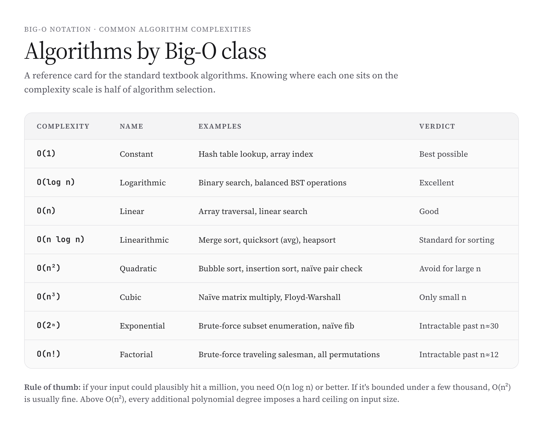
A quick mental reference for the algorithms you’ll meet most often:

• \(O(1)\): hash table operations, array indexing, stack/queue push/pop, doubly linked list insert/delete given pointer.
• \(O(\log n)\): binary search, balanced BST operations, heap insert/delete-min, exponentiation by squaring.
• \(O(n)\): array traversal, linear search, building a heap, single graph traversal step.
• \(O(n \log n)\): merge sort, heapsort, quicksort (average), FFT, kd-tree construction.
• \(O(n^2)\): bubble sort, insertion sort, selection sort, naive nearest-neighbor brute force.
• \(O(n^3)\): naive matrix multiply, Floyd-Warshall all-pairs shortest paths, naive 3D point cloud algorithms.
• \(O(2^n)\): brute-force subset enumeration, naive recursive Fibonacci, NP-hard exact algorithms.
• \(O(n!)\): brute-force traveling salesman, all-permutation enumeration.

Why Constants Matter in Practice (Even Though Big-O Ignores Them)

Big-O ignores constants for theoretical tidiness, but constants matter enormously in practice. An \(O(n \log n)\) algorithm with constant 1000 might be slower than an \(O(n^2)\) algorithm with constant 1 for small inputs. The crossover happens at the \(n\) where \(1000 \cdot n \log n = n^2\), which is around \(n \approx 10{,}000\).

This is why insertion sort beats quicksort for very small arrays (production sort implementations switch to insertion sort below \(n \approx 10\) or so). It’s also why constant-factor improvements (“optimization”) matter for hot code paths even when the asymptotic complexity is unchanged.

Common Mistakes With Big-O

1. Treating Big-O as exact runtime. Big-O describes asymptotic behavior; actual runtime depends on constants, hardware, and inputs. \(O(n)\) doesn’t mean “linear in milliseconds” — it means linear in operation count, asymptotically.
2. Ignoring lower-order terms when they matter. For small inputs, lower-order terms dominate. Big-O is a long-run prediction, not a short-run guarantee.
3. Confusing time and space complexity. An algorithm can be fast and memory-hungry, or slow and memory-efficient. Always specify which.
4. Conflating average and worst case. “Quicksort is \(O(n \log n)\)” is the average case. The worst case is \(O(n^2)\), which can matter for adversarial inputs.
5. Reading nested loops as automatic \(O(n^2)\). Two nested loops over different ranges might be \(O(n + m)\), not \(O(n m)\). Read the actual iteration counts.
6. Misjudging recursive complexity. Recursive algorithms need recurrence-relation analysis (Master theorem, recursion tree). Eyeballing the code often produces wrong complexity estimates.

A Brief History of Big-O Notation

Big-O notation predates computer science. German mathematician Paul Bachmann introduced it in 1894 in his treatise on number theory, and Edmund Landau popularized it in 1909. The original use was in analytic number theory for describing the asymptotic growth of error terms in approximations.

Donald Knuth introduced Big-O to computer science in his The Art of Computer Programming series, starting in the 1960s and 1970s. Knuth’s adoption made Big-O the standard language for algorithm analysis, replacing earlier ad-hoc notations.

Today every undergraduate computer science curriculum teaches Big-O analysis. Coding interviews universally test it. Algorithm research papers use it as the basic vocabulary for comparing performance. After 130+ years, Big-O remains the dominant framework for asymptotic analysis across mathematics and computer science.

The Master Theorem

For divide-and-conquer recurrences of the form \(T(n) = aT(n/b) + f(n)\), the master theorem gives the asymptotic complexity directly:

• If \(f(n) = O(n^{\log_b a – \epsilon})\) for some \(\epsilon > 0\): \(T(n) = \Theta(n^{\log_b a})\).
• If \(f(n) = \Theta(n^{\log_b a})\): \(T(n) = \Theta(n^{\log_b a} \log n)\).
• If \(f(n) = \Omega(n^{\log_b a + \epsilon})\) and the regularity condition holds: \(T(n) = \Theta(f(n))\).

The master theorem covers most divide-and-conquer recurrences (merge sort, quicksort, binary search, fast Fourier transform). For recurrences that don’t fit, recursion-tree analysis or substitution proofs handle the general case.

P vs NP and Computational Complexity Classes

Beyond Big-O, computational complexity theory groups problems into classes by inherent difficulty. P is the class of problems solvable in polynomial time. NP is the class where solutions can be verified in polynomial time. The famous P vs NP question asks whether every problem with a quickly-checkable solution can also be quickly solved.

NP-complete problems (traveling salesman, satisfiability, graph coloring) are the hardest in NP — if any NP-complete problem has a polynomial-time algorithm, all NP problems do. Most computer scientists believe P ≠ NP, but no proof exists. The question remains one of the seven Millennium Prize Problems with a $1 million reward for resolution.

Worked Example: Recursive Complexity Analysis

Analyze the complexity of merge sort. The recurrence is \(T(n) = 2T(n/2) + O(n)\) — two recursive calls on halves plus a linear merge step.

By the master theorem with \(a = 2, b = 2, f(n) = O(n)\): \(\log_b a = 1\), and \(f(n) = \Theta(n^1)\) matches the boundary case. So \(T(n) = \Theta(n \log n)\). Merge sort runs in \(O(n \log n)\) time.

The same analysis applies to many divide-and-conquer algorithms: binary search (\(T(n) = T(n/2) + O(1)\), giving \(O(\log n)\)), Karatsuba multiplication (\(T(n) = 3T(n/2) + O(n)\), giving \(O(n^{\log_2 3})\)), and the FFT (\(T(n) = 2T(n/2) + O(n)\), giving \(O(n \log n)\)).

When Big-O Is Misleading

Big-O ignores constants and lower-order terms. For real-world inputs, those can dominate. Three classic cases where Big-O misleads:

• Galactic algorithms: \(O(n \log \log n)\) integer multiplication is asymptotically faster than \(O(n \log n)\) FFT-based multiplication, but the constants are so large that no practical input triggers the crossover.
• Cache effects: two \(O(n^2)\) algorithms can have wildly different real-world speeds depending on memory access patterns. Cache-friendly traversal beats cache-hostile traversal by 10×–100×.
• Small inputs: for \(n < 30\), insertion sort beats quicksort despite the worse asymptotic complexity. Production sort routines hybridize for this reason.

Big-O is the right tool for choosing between fundamentally different algorithm classes. For optimizing within a class, you need profiling, benchmarks, and an understanding of the underlying hardware.

Worked Example: Analyzing Two-Sum

The classic interview problem: given an array and a target, find two indices whose values sum to the target. Two solutions:

Brute force: nested loop over all pairs. Each pair is checked in \(O(1)\); there are \(\binom{n}{2} \approx n^2/2\) pairs. Total: \(O(n^2)\) time, \(O(1)\) space.

Hash table: single pass through the array. For each element \(x\), check whether \(\text{target} – x\) is already in a hash table; if so, found the pair. Otherwise add \(x\) to the hash table. Each iteration is \(O(1)\) average; total iterations: \(n\). Total: \(O(n)\) time, \(O(n)\) space.

The hash-table version trades extra memory for dramatically better runtime. For \(n = 10^6\), brute force does \(5 \times 10^{11}\) operations (hours). The hash version does \(10^6\) operations (milliseconds). This is the textbook lesson on space-time trade-offs in algorithm design.

Common Cheat Sheet: Big-O for Standard Data Structures

Most data structures have characteristic complexities for their main operations. A quick reference:

• Array: indexed access \(O(1)\); search \(O(n)\); insert/delete at end \(O(1)\) amortized; insert/delete in middle \(O(n)\).
• Linked list: indexed access \(O(n)\); search \(O(n)\); insert/delete with pointer \(O(1)\).
• Hash table: insert, lookup, delete all \(O(1)\) average, \(O(n)\) worst case.
• Balanced BST (red-black, AVL): insert, lookup, delete all \(O(\log n)\) worst case.
• Heap: peek minimum \(O(1)\); insert and extract-minimum \(O(\log n)\).
• Stack/queue: push, pop, peek all \(O(1)\).
• Trie: insert and search of a string of length \(k\) is \(O(k)\) — independent of total stored strings.

Knowing this table by heart lets you pick the right data structure for any problem in seconds. It’s the practical basis for algorithm selection.

How Different Languages Express Big-O

The asymptotic complexity of an algorithm is independent of programming language, but the constant factors aren’t. Python is typically 10-50× slower than C for the same algorithm, but a Python implementation of \(O(n \log n)\) sorting still beats a C implementation of \(O(n^2)\) sorting for large inputs.

This is why Big-O is the right tool for choosing algorithms across languages. A million-element sort in well-implemented Python merge sort takes seconds; a million-element sort in C bubble sort takes hours. The asymptotic class dominates language-specific constants for any non-trivial input size.

Big-O in Database Query Performance

Database queries have characteristic complexities. A full table scan is \(O(n)\). An indexed lookup on a B-tree is \(O(\log n)\). A nested-loop join is \(O(n \cdot m)\). A hash join is \(O(n + m)\) average case.

Query optimizers in databases (PostgreSQL, MySQL, BigQuery) compute estimated costs for different execution plans using Big-O reasoning combined with row-count statistics. Understanding the asymptotic complexity of indexes, joins, and aggregations is what separates working DBAs from struggling ones. EXPLAIN plans show you exactly which complexity class each operation uses.

FAQs