Chain Rule

The chain rule is the technique for differentiating composite functions — functions inside other functions. It’s the workhorse rule of calculus. Once nested functions show up (and they show up everywhere in physics, economics, and machine learning), no other rule gets you through.

The chain rule trips students up because it’s easy to forget the inner derivative. The fix is a clean mental recipe: differentiate the outer function, leave the inner alone, then multiply by the derivative of the inner. Three steps, every time. Once it becomes automatic, the chain rule is the rule you reach for most often.

This study note covers the formula in both notations, the three-step recipe, why it works intuitively, multiple worked examples (including triple nesting), the multivariable generalization, the role of the chain rule in backpropagation and gradient descent, common mistakes, and a brief history.

Chain rule composition diagram and worked example modern textbook illustration

The Formula

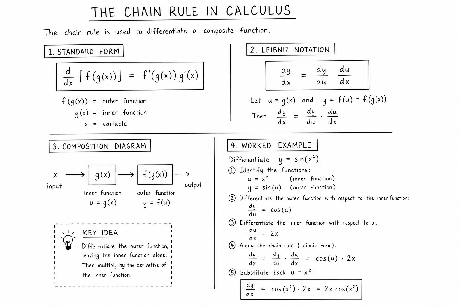
For a composite function $y = f(g(x))$:

$$\frac{dy}{dx} = f'(g(x)) \cdot g'(x)$$

In Leibniz notation, with $u = g(x)$:

$$\frac{dy}{dx} = \frac{dy}{du} \cdot \frac{du}{dx}$$

The Leibniz form is suggestive: differentials behave like fractions, with the $du$ cancelling. They aren’t literal fractions, but the bookkeeping works out for many practical purposes (separable differential equations, related rates problems, change of variables in integrals).

The Three-Step Recipe

Identify the outer and inner functions. The outer is what you see “first” if you read left to right; the inner is what’s being plugged in.
Differentiate the outer, leaving the inner intact.
Multiply by the derivative of the inner.

For $\sin(x^2)$: outer is $\sin(\cdot)$, inner is $x^2$. Step 2 gives $\cos(x^2)$. Step 3 multiplies by $2x$. Result: $\cos(x^2) \cdot 2x = 2x \cos(x^2)$.

Repeating this recipe until it becomes automatic is the single highest-leverage thing you can do as a calculus student. Every other technique builds on it, including implicit differentiation, related rates, and most of multivariable calculus.

Why It Works (Intuition)

If $u$ changes by a small amount $\Delta u$, then $y$ changes by approximately $(dy/du) \cdot \Delta u$. And if $x$ changes by $\Delta x$, then $u$ changes by approximately $(du/dx) \cdot \Delta x$. Substituting, $y$ changes by $(dy/du)(du/dx) \Delta x$. Divide by $\Delta x$ and take the limit, and the chain rule falls out.

That’s the bookkeeping for “rates compose multiplicatively.” A 5% change in something, times a 3% sensitivity to that something, gives a 0.15% change in the final output. That’s chain rule arithmetic in everyday percent terms.

Worked Examples

Exponential composition:

$$\frac{d}{dx} e^{3x^2 + 1} = e^{3x^2 + 1} \cdot 6x$$

Logarithmic composition:

$$\frac{d}{dx} \ln(\cos x) = \frac{1}{\cos x} \cdot (-\sin x) = -\tan x$$

Triple nesting:

$$\frac{d}{dx} \sin(\cos(x^2)) = \cos(\cos(x^2)) \cdot (-\sin(x^2)) \cdot 2x$$

For triple nesting, just apply the chain rule twice. Outer, middle, inner — chain them all together. The pattern extends to arbitrary depth: the derivative of $f_1(f_2(\ldots f_n(x)))$ is the product of derivatives at each layer evaluated at the appropriate inner expression.

Power of a polynomial:

$$\frac{d}{dx} (3x^2 + 5x + 1)^7 = 7(3x^2 + 5x + 1)^6 \cdot (6x + 5)$$

The Multivariable Chain Rule

For a function $z = f(x, y)$ where $x = g(t)$ and $y = h(t)$:

$$\frac{dz}{dt} = \frac{\partial z}{\partial x} \frac{dx}{dt} + \frac{\partial z}{\partial y} \frac{dy}{dt}$$

Each variable $z$ depends on contributes a partial derivative term. The full derivative sums all the contributions. This is the central tool for related-rates problems in multiple variables, transformations in fluid mechanics, and tracking how outputs change as multiple inputs all evolve.

The matrix version is even cleaner. For a vector function $\mathbf{F}(\mathbf{G}(x))$:

$$\mathbf{J}_{\mathbf{F} \circ \mathbf{G}}(x) = \mathbf{J}_{\mathbf{F}}(\mathbf{G}(x)) \cdot \mathbf{J}_{\mathbf{G}}(x)$$

The Jacobian of the composition equals the product of the Jacobians. This matrix form is the foundation for backpropagation in neural networks.

Backpropagation as Chain Rule

A neural network is a deeply nested composition of functions: each layer applies a linear transformation followed by a nonlinear activation. To train the network, you compute the gradient of the loss with respect to every weight, and you do it by repeated chain rule application.

Backpropagation is the algorithm that performs this computation efficiently. Forward pass: compute outputs layer by layer. Backward pass: starting from the loss, compute gradients layer by layer using the chain rule, multiplying local Jacobians as you go. The forward and backward computations have the same complexity, which is why training neural networks is feasible at scale.

Without the chain rule, training deep networks is intractable. Frameworks like PyTorch, TensorFlow, and JAX implement automatic differentiation by tracking computational graphs and applying the chain rule symbolically. Read more in best machine learning courses.

Implicit Differentiation as Chain Rule

Implicit differentiation uses the chain rule to find $dy/dx$ when $y$ is defined implicitly by an equation. Differentiate both sides with respect to $x$, treating $y$ as a function of $x$ and applying the chain rule wherever $y$ appears.

Example: differentiate $x^2 + y^2 = 25$ (a circle).

$$2x + 2y \cdot \frac{dy}{dx} = 0 \implies \frac{dy}{dx} = -\frac{x}{y}$$

The $2y \cdot dy/dx$ is the chain rule in action: differentiating $y^2$ with respect to $x$ gives $2y$ (outer) times $dy/dx$ (inner derivative).

This trick handles equations that can’t be solved cleanly for $y$, such as $\sin(xy) + e^{x+y} = x^2$. Implicit differentiation also produces derivatives of inverse functions efficiently — the derivative of $\arcsin x$ is derived this way.

Related rates problems use the chain rule to find how one quantity’s rate of change relates to another’s. Standard format: a geometric or physical relationship connects two or more variables, and you’re given the rate of change of one and asked for the rate of change of another.

Example: a balloon is inflated at 5 cubic feet per minute. How fast is the radius growing when the balloon is 10 feet across?

Volume $V = \frac{4}{3}\pi r^3$. Differentiate both sides with respect to $t$:

$$\frac{dV}{dt} = 4\pi r^2 \cdot \frac{dr}{dt}$$

Plug in $dV/dt = 5$ and $r = 5$: $5 = 100\pi (dr/dt)$, so $dr/dt = 1/(20\pi)$ feet per minute. The chain rule converted “volume change” into “radius change” through the geometric relationship.

Where the Chain Rule Lives in Practice

Physics: velocity components, related rates, Lagrangian mechanics, every coordinate transformation.
Probability: change-of-variable formulas for densities (the Jacobian factor is exactly the chain rule).
Economics: elasticity calculations involving demand, price, and quantity.
Machine learning: backpropagation IS the chain rule applied across thousands of layers.
Differential equations: separable equations rely on chain-rule reasoning.
Engineering: sensitivity analysis through compound systems, control theory, signal processing chains.
Computer graphics: rendering pipelines that compose transforms and shaders are differentiated through the chain rule for differentiable rendering.

If you ever wondered why the chain rule gets so much airtime in calculus class, the answer is that downstream subjects depend on it harder than they depend on any other rule.

Common Mistakes

Forgetting the inner derivative. The most common mistake. Leaving off the $g'(x)$ factor turns the chain rule into the wrong rule.
Confusing the chain rule with the product rule. Chain rule is for compositions $f(g(x))$. Product rule is for products $f(x) g(x)$. They look similar in passing but apply to different structures.
Misidentifying the outer function. For $\sin^2(x)$, the outer is the squaring, not the sine. Rewrite as $(\sin x)^2$ and the chain rule gives $2 \sin x \cdot \cos x$.
Applying the chain rule when not needed. If the function isn’t a composition (just $\sin x$, no inner function), you don’t need the chain rule. Differentiate directly.
Stopping after one layer in deeply nested expressions. Triple nesting needs the chain rule applied twice, not once. Each layer contributes its own derivative.

Worked Example: Differentiating a Logistic Function

The logistic (sigmoid) function $\sigma(x) = 1/(1 + e^{-x})$ is everywhere in machine learning and probability. Its derivative is famously elegant: $\sigma'(x) = \sigma(x)(1 – \sigma(x))$.

Derivation by chain rule. Rewrite as $\sigma(x) = (1 + e^{-x})^{-1}$. Apply chain rule:

$$\sigma'(x) = -1 \cdot (1 + e^{-x})^{-2} \cdot (-e^{-x}) = \frac{e^{-x}}{(1 + e^{-x})^2}$$

Now factor: multiply top and bottom by $\sigma(x) = 1/(1+e^{-x})$, and you get $\sigma'(x) = \sigma(x) (1 – \sigma(x))$. The clean form is what makes sigmoid neurons easy to backpropagate through.

History of the Chain Rule

The chain rule was implicit in Newton’s and Leibniz’s original calculus work. Leibniz’s notation $dy/dx$ practically begs the chain rule into existence — the suggestive cancellation of $du$ made the rule feel natural and easy to remember. Newton’s fluxion approach worked but didn’t lend itself to the same intuitive notation.

Cauchy formalized the chain rule rigorously in the 1820s as part of the broader effort to put calculus on epsilon-delta foundations. The multivariable version was developed throughout the 19th century alongside the rest of multivariable calculus.

The 20th century brought the chain rule into machine learning. Backpropagation (Rumelhart, Hinton, Williams, 1986) is just the chain rule applied across neural network layers. Automatic differentiation (Wengert, 1964) generalizes it across arbitrary computational graphs. Today, every deep learning framework treats efficient chain rule computation as its central engineering challenge.

Related rates problems use the chain rule to translate one rate of change into another through a geometric or physical relationship. Standard format: a constraint links two variables, you know one rate, you need the other.

Example: a 13-foot ladder leans against a wall. The bottom slides outward at 2 ft/s. How fast does the top slide down when the bottom is 5 feet from the wall?

Constraint: $x^2 + y^2 = 169$. Differentiate both sides with respect to time: $2x \frac{dx}{dt} + 2y \frac{dy}{dt} = 0$. At $x = 5$, $y = 12$. Plug in $dx/dt = 2$: $2(5)(2) + 2(12) \frac{dy}{dt} = 0$, so $dy/dt = -5/6$ ft/s. The negative sign indicates the top is descending.

Related rates problems are essentially chain-rule arithmetic with a geometric setup; the technique generalizes to fluid dynamics, mechanical linkages, and engineering control problems.

Chain Rule for Higher Derivatives

The second derivative of a composite function involves multiple chain-rule applications. For $y = f(g(x))$:

$$\frac{d^2 y}{dx^2} = f”(g(x)) \cdot (g'(x))^2 + f'(g(x)) \cdot g”(x)$$

Notice the product rule appears on top of the chain rule because we’re differentiating $f'(g(x)) \cdot g'(x)$. Higher derivatives of compositions get progressively more complex; Faà di Bruno’s formula gives the general expression.

Chain Rule in Information Theory

Mutual information satisfies a chain rule: $I(X; Y, Z) = I(X; Y) + I(X; Z | Y)$. Entropy satisfies $H(X, Y) = H(X) + H(Y | X)$. These information-theoretic chain rules are formal analogues of the calculus chain rule and underpin source coding, channel capacity, and modern compression algorithms.

Faà di Bruno’s Formula

For the $n$-th derivative of a composition:

$$\frac{d^n}{dx^n} f(g(x)) = \sum_{\pi \in \Pi_n} f^{(|\pi|)}(g(x)) \prod_{B \in \pi} g^{(|B|)}(x)$$

where the sum runs over all partitions $\pi$ of $\{1, \ldots, n\}$. Faà di Bruno’s formula generalizes the chain rule to any order and is the closed-form answer to “what’s the $n$-th derivative of a composition?”

The formula is rarely used by hand but is essential in symbolic computation and combinatorial analysis. It also clarifies why higher derivatives of composite functions grow so quickly in algebraic complexity.

Worked Example: Differentiating a Composite Polynomial

Differentiate $f(x) = (x^3 + 5x – 2)^4$. Outer function is $(\cdot)^4$, inner is $x^3 + 5x – 2$. Apply chain rule:

$$f'(x) = 4(x^3 + 5x – 2)^3 \cdot (3x^2 + 5)$$

Without the chain rule you’d have to expand the polynomial first (tedious for the fourth power) and then differentiate. The chain rule turns a 60-second algebra problem into a 5-second one.

Chain Rule and Probability Density Transformations

If $Y = g(X)$ is a smooth invertible transformation of a random variable, the density of $Y$ is related to the density of $X$ by:

$$f_Y(y) = f_X(g^{-1}(y)) \left|\frac{d}{dy} g^{-1}(y)\right|$$

The Jacobian factor is exactly the chain rule applied to the change of variables. This formula is the foundation for working with derived random variables, change-of-coordinate formulas in statistics, and normalizing flow models in deep learning.

Memorizing the Chain Rule by Pattern

Most students who struggle with the chain rule struggle because they treat it as a formula to memorize rather than a structural recognition exercise. The fix: train yourself to spot composite functions on sight before reaching for any formula. $\sin(x^2)$, $e^{3x+1}$, $\sqrt{x^2 + 4}$, $\ln(\cos x)$, $(2x + 1)^5$ — all composite. Practice identifying outer and inner pairs in 100 examples and the formula becomes automatic.

This is the same principle behind learning chess openings or recognizing musical keys: structural pattern recognition trumps mechanical formula application. Once recognition is automatic, the chain rule stops being a step in your derivative process and becomes a built-in instinct.

Why the Chain Rule Has No Quotient-Rule Analogue

You might wonder: if there’s a chain rule for compositions and a product rule for products, is there a “chain rule for quotients”? The answer is no, because the quotient rule already handles the case via the product and chain rules combined: $f/g = f \cdot g^{-1}$, and differentiating using product rule plus chain rule gives the standard quotient rule.

This is a small but important point: the basic differentiation rules form a minimal complete set. Power rule + sum rule + product rule + chain rule generate every other rule you’ll meet in single-variable calculus. The quotient rule is convenient shorthand but not logically primitive.

Chain Rule and Differential Operators

The chain rule extends to differential operators. The Laplacian $\Delta f = \nabla^2 f$ under coordinate transformations transforms via the chain rule. The change from Cartesian to polar (or spherical) coordinates introduces extra terms that account for the curvature of the coordinate system — all derivable through systematic chain rule application.

This is why physics textbooks contain so many “Laplacian in spherical coordinates” derivations. The underlying math is repeated chain-rule applications across an orthogonal coordinate transformation, with Jacobian factors and metric tensors keeping track of the geometry.

FAQs

When do I need to use the chain rule?

Whenever the function is a composition — one function plugged into another. If you can write the function as f(g(x)), the chain rule applies. Examples: sin(x²), e^(3x), √(x² + 1), ln(tan x). If there’s no nesting, no chain rule.

How do I identify outer and inner functions?

The outer function is what you’d evaluate last if you computed step by step. The inner function is what you’d evaluate first. For sin(x²), you’d compute x² first then take sin, so x² is inner and sin is outer.

What’s the chain rule for three or more nested functions?

Apply the chain rule iteratively. For y = f(g(h(x))): dy/dx = f'(g(h(x))) · g'(h(x)) · h'(x). Each layer contributes its own derivative; multiply them all together.

Is the chain rule the same as the product rule?

No. The product rule is for products of functions: (fg)’ = f’g + fg’. The chain rule is for compositions: (f∘g)’ = f'(g) · g’. Both involve two functions, but they apply in different situations and produce different results.

How is backpropagation related to the chain rule?

Backpropagation in neural networks is the chain rule applied repeatedly across layers. The gradient of the loss with respect to early weights is computed by chaining derivatives through each subsequent layer. Without the chain rule, training deep networks would be intractable.

What’s the multivariable chain rule?

For z = f(x, y) where x and y both depend on t, dz/dt = (∂z/∂x)(dx/dt) + (∂z/∂y)(dy/dt). Each input variable contributes a partial derivative term, summed together. The matrix form generalizes to vector-valued functions through Jacobian multiplication.

Why does the chain rule have an outer derivative and an inner derivative?

Because the rate of change of a composition is the product of the rates of change at each layer. If the outer function changes 3 units per unit of inner, and the inner changes 2 units per unit of input, the composition changes 6 units per unit of input — outer rate times inner rate.

What is implicit differentiation and how does it use the chain rule?

Implicit differentiation finds dy/dx when y is defined implicitly by an equation. Differentiate both sides with respect to x, applying the chain rule wherever y appears. The result expresses dy/dx in terms of both x and y.

Can I use the chain rule for integration?

Yes — substitution is the chain rule run in reverse. Whenever you spot a function and its derivative both present in the integrand, substitution recovers the original function. Recognizing chain-rule structures is what makes substitution work.

What’s a Jacobian and how does it relate to the chain rule?

The Jacobian is a matrix of partial derivatives for vector-valued multivariable functions. The chain rule for compositions of vector functions is a Jacobian multiplication: J(f∘g) = J(f) · J(g). This is the central operation in automatic differentiation and backpropagation.

Why is the chain rule taught after the basic rules?

Because most non-trivial functions are compositions, and the chain rule is the first technique that requires careful identification of structure. Earlier rules (power, sum, product) operate on visible structure; the chain rule requires recognizing implicit composition. It’s the conceptual jump from mechanical to structural differentiation.

How does automatic differentiation handle the chain rule?

Automatic differentiation tracks the computational graph of a function as it’s evaluated. Each node knows its local derivative. Backward through the graph, AD multiplies local derivatives via the chain rule to assemble the full gradient. This is exact (not numerical) and scales linearly in the number of operations.

What’s the chain rule for second derivatives?

It’s the chain rule applied twice with a product rule in the middle: d²/dx² f(g(x)) = f”(g(x)) · (g'(x))² + f'(g(x)) · g”(x). The general formula for the n-th derivative is Faà di Bruno’s formula, which involves a sum over set partitions.

How are related rates and the chain rule connected?

Related rates problems are chain-rule applications dressed up as physical scenarios. A geometric or physical constraint links two or more variables; differentiating both sides with respect to time uses the chain rule to relate the rates of change of those variables.