Differential Equation

Q: Why do differential equations need initial conditions?

Because the equation alone has infinitely many solutions. dy/dx = ky has solutions y = c·e^(kx) for any constant c. The initial condition (e.g., y(0) = 5) pins down which specific solution applies. First-order ODEs need 1 initial condition; second-order need 2; an nth-order ODE needs n.

Q: How do you solve a differential equation that has no closed-form solution?

Numerically. Replace derivatives with finite differences and step through the variable computationally. Euler's method is the simplest (and least accurate); Runge-Kutta (RK4) is the workhorse for ODEs. Modern numerical libraries (scipy.integrate.solve_ivp, MATLAB's ode45, Wolfram Mathematica) handle the details. Most real-world physics, engineering, and biology problems are solved this way because closed-form solutions don't exist.

A differential equation is an equation that relates a function to its derivatives. They describe how things change, which makes them the natural language of physics, engineering, biology, economics, and essentially every quantitative field. Newton’s laws are differential equations. Maxwell’s equations are differential equations. Population dynamics, chemical reaction rates, electric circuits, heat flow, sound waves, financial derivatives — all start as differential equations. Solving them is what calculus, in a sense, is for.

Differential equation illustration — A first-order differential equation dy/dx = ky and its exponential solution y = y_0 e^(kx).

What a Differential Equation Is

A differential equation contains derivatives of an unknown function. The simplest example:

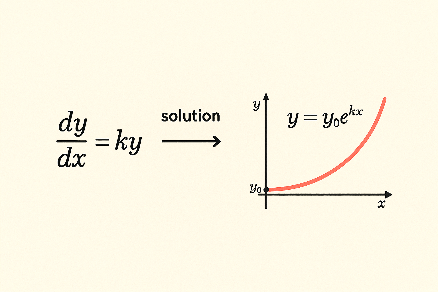
$$ \frac{dy}{dx} = k y $$

This says: ‘the rate of change of \$ y \$ with respect to \$ x \$ is proportional to \$ y \$ itself.’ Solving it means finding the function \$ y(x) \$ that satisfies the equation. In this case, the solution is the exponential:

$$ y(x) = y_0 e^{kx} $$

where \$ y_0 \$ is the value of \$ y \$ at \$ x = 0 \$. You can verify by differentiating: \$ dy/dx = k y_0 e^{kx} = k y \$. ✓

Order and Linearity

Differential equations are classified by two main properties:

Order = the highest derivative that appears. \$ dy/dx = ky \$ is first-order. \$ d^2y/dx^2 + 4y = 0 \$ is second-order. Newton’s second law \$ F = m \\frac{d^2x}{dt^2} \$ is also second-order.
Linearity — a differential equation is LINEAR if the unknown function and its derivatives appear only to the first power and not multiplied together. Otherwise it’s nonlinear. Linear equations have nice properties (superposition, closed-form solutions, predictable behavior). Nonlinear equations are harder and can exhibit chaos.

Ordinary vs Partial

Two big subdivisions of the differential equation universe.

Ordinary differential equations (ODEs) involve a single independent variable (usually time, often denoted t, or position, denoted x). The unknown is a function of one variable. Newton’s laws for a particle on a line are ODEs.
Partial differential equations (PDEs) involve multiple independent variables. The unknown is a function of several variables, and derivatives are partial. The heat equation, wave equation, and Maxwell’s equations are PDEs. Much harder to solve in general.

Three Canonical First-Order ODEs

Exponential growth/decay

$$ \frac{dy}{dx} = k y \implies y(x) = y_0 e^{kx} $$

Models: bank interest, population growth, radioactive decay, drug elimination from the body, RC circuit discharge.

Logistic growth (population with carrying capacity)

$$ \frac{dy}{dx} = k y \left(1 – \frac{y}{K}\right) $$

Solution is an S-shaped curve approaching the carrying capacity \$ K \$. Models population dynamics under resource limits, technology adoption, epidemic spread (early phase), and many other ‘limit to growth’ phenomena.

Newton’s law of cooling

$$ \frac{dT}{dt} = -k (T – T_{env}) $$

The rate at which an object’s temperature \$ T \$ approaches the environment temperature \$ T_{env} \$ is proportional to the temperature difference. Solution is an exponentially decaying difference.

Second-Order: The Pendulum and Spring

Newton’s second law \$ F = ma = m \\ddot{x} \$ is naturally second-order. For a mass on a spring with restoring force \$ F = -kx \$:

$$ m \frac{d^2 x}{dt^2} = -kx \implies \frac{d^2 x}{dt^2} + \omega^2 x = 0 $$

where \$ \\omega = \\sqrt{k/m} \$. The general solution is \$ x(t) = A \\cos(\\omega t) + B \\sin(\\omega t) \$, or equivalently \$ x(t) = C \\cos(\\omega t + \\varphi) \$ — simple harmonic motion. The same equation describes pendulums (small angles), LC circuits, and molecular vibrations.

Add damping (a friction-like term proportional to velocity) and the equation becomes \$ \\ddot{x} + 2\\gamma \\dot{x} + \\omega^2 x = 0 \$. The solutions depend on the damping ratio: under-damped (oscillates while decaying), critically damped (fastest return to rest without overshoot), or over-damped (slow exponential return). Critical damping is the design target for car shock absorbers and door closers.

Initial Conditions and Boundary Conditions

A differential equation has infinitely many solutions in general. To pick one specific solution, you need additional information.

Initial conditions specify the function value (and possibly its derivatives) at one point. For first-order ODEs, you need 1 initial condition (e.g., \$ y(0) = 5 \$). For second-order, 2 (e.g., \$ x(0) = A \$, \$ \\dot{x}(0) = 0 \$).
Boundary conditions specify values at multiple points (often the boundaries of the spatial domain for PDEs). E.g., the temperature at both ends of a metal rod.

An ODE plus its initial conditions is called an initial value problem (IVP); a PDE plus boundary conditions is a boundary value problem (BVP). Both have well-developed solution theories.

When You Can’t Solve Analytically

Most differential equations have no closed-form solution. For these, numerical methods take over. The basic idea: replace derivatives with finite differences and step through time computationally.

Euler’s method — the simplest. Step forward by a small $ \Delta x $ using the current derivative. Fast but inaccurate.
Runge-Kutta methods (RK4 in particular) — much more accurate. The workhorse of numerical ODE solving.
Adaptive methods — adjust step size based on local error estimates. What scipy.integrate.solve_ivp does by default.
Finite element methods (FEM) — for PDEs. Discretize the spatial domain into elements and solve the resulting algebraic system.

Modern computational physics and engineering depend completely on numerical differential equation solvers. Weather prediction, fluid dynamics simulations, structural analysis, drug pharmacokinetics — all are numerical PDE/ODE problems at the core.

Frequently Asked Questions

What is a differential equation?

A differential equation is an equation that relates a function to its derivatives. The simplest example, dy/dx = ky, says the rate of change of y is proportional to y itself. Solving means finding the function y(x) that satisfies the equation. Differential equations are the natural language for describing how things change over time or space.

What’s the difference between ordinary and partial differential equations?

Ordinary differential equations (ODEs) involve a single independent variable — usually time or position — and the unknown is a function of one variable. Partial differential equations (PDEs) involve multiple independent variables (e.g., position AND time), and the unknown is a function of all of them. PDEs are generally much harder to solve.

What does the order of a differential equation mean?

Order is the highest derivative that appears in the equation. dy/dx = ky is first-order (only first derivatives). Newton’s second law F = m d²x/dt² is second-order (involves the second derivative). Higher-order equations need more initial conditions to pin down a unique solution.

What is exponential growth as a differential equation?

dy/dx = ky, where k > 0, models exponential growth — the rate of change is proportional to the current value. The solution is y(x) = y_0 e^(kx), where y_0 is the value at x = 0. The same equation with k < 0 models exponential decay. This single equation describes bank interest, population growth, radioactive decay, drug elimination, and many other processes.

Why do differential equations need initial conditions?

Because the equation alone has infinitely many solutions. dy/dx = ky has solutions y = c·e^(kx) for any constant c. The initial condition (e.g., y(0) = 5) pins down which specific solution applies. First-order ODEs need 1 initial condition; second-order need 2; an nth-order ODE needs n.

How do you solve a differential equation that has no closed-form solution?

Numerically. Replace derivatives with finite differences and step through the variable computationally. Euler’s method is the simplest (and least accurate); Runge-Kutta (RK4) is the workhorse for ODEs. Modern numerical libraries (scipy.integrate.solve_ivp, MATLAB’s ode45, Wolfram Mathematica) handle the details. Most real-world physics, engineering, and biology problems are solved this way because closed-form solutions don’t exist.