Derivatives in Calculus

The derivative in calculus is the instantaneous rate of change of a function. Geometrically, it’s the slope of the tangent line at a point. Physically, it’s velocity if the function is position, or acceleration if the function is velocity. Economically, it’s marginal cost or marginal revenue. The derivative shows up anywhere a quantity changes and you want to know how fast.

Most of single-variable calculus is built on three ideas: the limit definition, a small set of rules for differentiating common functions, and the chain rule. Memorize those, and 90% of derivative problems become routine. The interesting work happens at the edges — non-differentiable points, optimization at constraint boundaries, and the derivative-driven core of modern machine learning and physics.

This study note covers the limit definition, notation conventions, the standard rules (power, product, quotient, chain), worked examples, what derivatives mean in real-world problems, optimization, the second derivative test, common pitfalls, and the historical and modern context.

The Limit Definition

The derivative of \(f\) at \(x\) is:

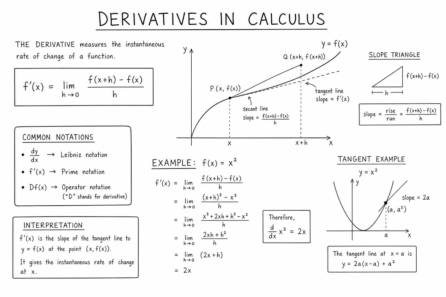
$$f'(x) = \lim_{h \to 0} \frac{f(x+h) – f(x)}{h}$$

The fraction is the average rate of change between \(x\) and \(x + h\) — the slope of the secant line through the two points. As \(h\) shrinks toward zero, the secant becomes the tangent, and the average rate becomes the instantaneous rate.

The derivative exists at \(x\) only when this limit exists. Sharp corners, vertical tangents, and discontinuities all kill differentiability. The function \(f(x) = |x|\) is continuous everywhere but not differentiable at \(x = 0\), where the left and right slopes disagree (-1 and +1, respectively).

Notation Conventions

The same idea has many costumes:

• Lagrange: \(f'(x)\), \(f”(x)\), \(f^{(n)}(x)\) — compact for general use
• Leibniz: \(\frac{dy}{dx}\), \(\frac{d^2y}{dx^2}\) — clear about what’s being differentiated with respect to what; mandatory for the chain rule
• Newton: \(\dot{y}\), \(\ddot{y}\) — mostly physics, dots mean derivatives with respect to time
• Operator: \(D_x f\) or \(\frac{d}{dx} f\) — useful in differential equations

Pick whichever the textbook uses; they all mean the same thing. Different fields developed different conventions because they emphasized different uses. Leibniz notation makes the chain rule feel like fraction cancellation. Newton’s dot notation keeps physics equations compact. Lagrange’s prime notation is the cleanest for general algebraic work.

The Rules You’ll Actually Use

From the limit definition you derive a small toolkit:

• Power rule: \(\frac{d}{dx} x^n = n x^{n-1}\) for any real \(n\)
• Constant rule: \(\frac{d}{dx} c = 0\)
• Sum rule: \((f + g)’ = f’ + g’\)
• Product rule: \((fg)’ = f’g + fg’\)
• Quotient rule: \(\left(\frac{f}{g}\right)’ = \frac{f’g – fg’}{g^2}\)
• Chain rule: \(\frac{d}{dx} f(g(x)) = f'(g(x)) g'(x)\)

Plus the standard library: \(\frac{d}{dx} \sin x = \cos x\), \(\frac{d}{dx} \cos x = -\sin x\), \(\frac{d}{dx} e^x = e^x\), \(\frac{d}{dx} \ln x = \frac{1}{x}\), \(\frac{d}{dx} \tan x = \sec^2 x\). Memorize these and you can differentiate nearly anything algebraically.

Worked Examples

Polynomial: Differentiate \(f(x) = 3x^4 – 2x^2 + 5x – 7\):

$$f'(x) = 12x^3 – 4x + 5$$

Power rule term by term, constants drop out. Bread-and-butter polynomial differentiation.

Product: Differentiate \(g(x) = x^2 \sin x\):

$$g'(x) = 2x \sin x + x^2 \cos x$$

Product rule with \(f = x^2\) and \(g = \sin x\).

Chain: Differentiate \(h(x) = \sin(x^2)\):

$$h'(x) = \cos(x^2) \cdot 2x = 2x \cos(x^2)\$$

Outer derivative \(\cos(\cdot)\) evaluated at the inner function, multiplied by inner derivative \(2x\).

What the Derivative Tells You

• Sign of \(f’\): positive means \(f\) is increasing, negative means decreasing.
• \(f’ = 0\): a critical point — possible local max, local min, or saddle.
• Sign of \(f”\): positive means \(f\) is concave up, negative means concave down.
• \(f” = 0\) with sign change: inflection point.

This is the toolkit behind optimization: find where \(f’ = 0\), check the second derivative, classify each critical point. It’s also how machine learning gradient descent works under the hood — read more in best machine learning courses and best data science courses.

The Second Derivative Test

For a critical point \(c\) where \(f'(c) = 0\):

• If \(f”(c) > 0\), then \(c\) is a local minimum.
• If \(f”(c) < 0\), then \(c\) is a local maximum.
• If \(f”(c) = 0\), the test is inconclusive — use the first-derivative sign chart or a higher-order test.

The test is fast for well-behaved functions. For \(f(x) = x^3\), the only critical point is at \(x = 0\); \(f”(0) = 0\), so the second-derivative test is inconclusive. Inspecting the sign of \(f’\) reveals \(x = 0\) is neither a max nor a min — it’s an inflection point where the tangent line crosses the curve.

For multivariable functions, the second-derivative test generalizes to the Hessian matrix. The eigenvalues of the Hessian classify critical points: all positive means local min, all negative means local max, mixed signs mean saddle. Quasi-Newton optimization methods (BFGS, L-BFGS) approximate the inverse Hessian to choose efficient search directions.

Implicit Differentiation

When a relationship between \(x\) and \(y\) isn’t explicitly solved for \(y\), differentiate both sides with respect to \(x\), treating \(y\) as a function of \(x\) and applying the chain rule wherever \(y\) appears.

Example: differentiate \(x^2 + y^2 = 25\) (the equation of a circle).

$$2x + 2y \frac{dy}{dx} = 0 \implies \frac{dy}{dx} = -\frac{x}{y}$$

Implicit differentiation handles equations that can’t be solved cleanly for \(y\), like \(\sin(xy) + e^{x+y} = x^2\). It also produces derivatives of inverse functions efficiently — the derivative of \(\arcsin x\) is derived this way from \(\sin y = x\).

Higher-Order Derivatives

The second derivative is the derivative of the derivative. The third derivative is the derivative of the second. And so on.

• If \(f(x) = \sin x\), then \(f'(x) = \cos x\), \(f”(x) = -\sin x\), \(f”'(x) = -\cos x\), \(f^{(4)}(x) = \sin x\). The pattern repeats with period 4.
• For \(f(x) = e^x\), all derivatives equal \(e^x\).
• For polynomials, the \(n\)-th derivative of \(x^n\) is \(n!\), and all higher derivatives are zero.

Higher-order derivatives appear in Taylor series, where they encode the local behavior of a function around a point. They also matter in physics: position is the original quantity, velocity is its derivative, acceleration is the second derivative, jerk is the third, snap is the fourth (yes, those are real names).

Differentiability vs Continuity

Differentiability is strictly stronger than continuity. Every differentiable function is continuous, but not every continuous function is differentiable.

Counterexamples:

• Sharp corners: \(|x|\) is continuous everywhere but not differentiable at 0.
• Vertical tangents: \(x^{1/3}\) has an infinite-slope tangent at 0, so the derivative doesn’t exist there.
• Cusps: functions like \(x^{2/3}\) have a cusp at 0, also non-differentiable.
• Pathological cases: the Weierstrass function is continuous everywhere but differentiable nowhere — a deeply counterintuitive example that motivated 19th-century rigor.

For practical work, almost every function you’ll meet is differentiable except at isolated points. Software-defined functions (neural network activations, splines, decision tree predictions) have known non-differentiable points that engineers handle deliberately.

Where Derivatives Live in Practice

• Physics: velocity, acceleration, force, related rates, Lagrangian and Hamiltonian mechanics. Most differential equations describe how physical quantities change over time or space.
• Economics: marginal cost, marginal revenue, marginal utility, elasticity. Almost every microeconomic optimization is a derivative-based problem.
• Engineering: stress-strain curves, signal processing (the derivative of position gives velocity, of voltage gives current through capacitors), control systems.
• Machine learning: gradient descent, backpropagation, automatic differentiation. Modern deep learning would not exist without efficient derivative computation across millions of parameters.
• Probability and statistics: probability density functions are derivatives of cumulative distribution functions; maximum likelihood estimation uses derivatives to find optimal parameters.
• Finance: option Greeks (delta, gamma, theta, vega) are derivatives of option prices with respect to underlying parameters.

Optimization in One Dimension

To find local maxima and minima of \(f(x)\) on an interval:

1. Compute \(f'(x)\).
2. Find critical points where \(f'(x) = 0\) or \(f’\) is undefined.
3. Apply the second-derivative test or first-derivative sign chart to classify each critical point.
4. Evaluate \(f\) at the critical points and the interval endpoints.
5. The largest value is the absolute max; the smallest is the absolute min.

This is the standard recipe in calculus textbooks and the foundation for nearly all classical optimization. Real-world problems usually have multiple local optima; finding the global optimum requires either exhaustive search of critical points or specialized algorithms (gradient descent with random restarts, simulated annealing, branch-and-bound for discrete cases).

Numerical Differentiation

When you can’t differentiate a function symbolically (no closed form, defined by data, or built from simulation), numerical differentiation approximates derivatives from function values.

Forward difference: \(f'(x) \approx (f(x+h) – f(x))/h\). Simple but only first-order accurate.

Central difference: \(f'(x) \approx (f(x+h) – f(x-h))/(2h)\). Second-order accurate, almost always preferred when both \(x+h\) and \(x-h\) are accessible.

Higher-order finite-difference schemes use more sample points and achieve fourth- or sixth-order accuracy. Automatic differentiation, used in modern ML frameworks, computes exact derivatives by tracking computational graphs and applying the chain rule symbolically — neither numerical nor purely symbolic, but a third approach that’s faster and more accurate than both.

A Brief History of Derivatives

Newton developed his version of calculus around 1665–1666, calling derivatives “fluxions” and using dot notation that survives in physics. Leibniz developed his version independently in the 1670s, using \(dy/dx\) notation that survives in nearly every other field. The bitter priority dispute that followed slowed mathematical progress in England for nearly a century, while continental Europe (using Leibniz’s notation) raced ahead.

The 19th century made derivatives rigorous. Cauchy and Weierstrass replaced infinitesimal arguments with limit-based definitions. By the 20th century, the limit-based derivative was the standard in textbooks worldwide. Nonstandard analysis in the 1960s rehabilitated infinitesimals on rigorous grounds, but the standard \(\varepsilon-\delta\) approach kept its dominance in education.

The modern era of derivatives is computational. Automatic differentiation transformed scientific computing in the 1980s–2000s and is now the foundation of every deep learning framework. Symbolic differentiation in computer algebra systems (Mathematica, SymPy) handles textbook problems instantly. The pencil-and-paper era is largely over for routine work; the conceptual understanding still matters because every technique builds on it.

Mean Value Theorem

If \(f\) is continuous on \([a, b]\) and differentiable on \((a, b)\), there exists \(c \in (a, b)\) such that:

$$f'(c) = \frac{f(b) – f(a)}{b – a}$$

Geometrically, somewhere between \(a\) and \(b\) the tangent line is parallel to the secant line. This is the workhorse theorem behind most existence results in single-variable calculus and the foundation for the Fundamental Theorem of Calculus.

Practical applications: if a car travels 100 miles in 2 hours, the MVT guarantees that at some moment the speedometer read exactly 50 mph. Speed cameras and average-speed enforcement use this principle: if your average speed exceeded the limit, MVT guarantees you exceeded the limit at some instant.

Derivatives of Inverse Functions

If \(f\) has an inverse \(f^{-1}\) and \(f'(f^{-1}(x)) \ne 0\), then:

$$\left(f^{-1}\right)'(x) = \frac{1}{f'(f^{-1}(x))}$$

This formula derives the standard inverse function derivatives. \(\frac{d}{dx} \arcsin x = 1/\sqrt{1 – x^2}\), \(\frac{d}{dx} \arctan x = 1/(1 + x^2)\), and \(\frac{d}{dx} \ln x = 1/x\) all come from applying this rule to standard functions.

Linear Approximation and Differentials

Near a point \(a\), a function is approximately linear: \(f(x) \approx f(a) + f'(a)(x – a)\). This is the linear approximation, and the difference \(dy = f'(a) dx\) is called the differential.

Linear approximation is the basis for Newton’s method (root-finding), error propagation in measurements, and first-order numerical analysis. The same idea generalizes to multivariable Taylor expansion and is the foundation for differential geometry.

Symbolic vs Numerical Differentiation

Symbolic differentiation manipulates algebraic expressions to produce closed-form derivatives. Computer algebra systems (Mathematica, SymPy, Maple) do this automatically. The output is exact and human-readable but can grow very large for complex expressions.

Numerical differentiation estimates derivatives from function evaluations using finite-difference formulas. It’s faster for one-off evaluations but accumulates floating-point error and only delivers approximate results.

Automatic differentiation, used in modern ML frameworks, is a third approach: it tracks the computational graph and applies the chain rule symbolically to each node, producing exact derivatives without ever simplifying the algebraic expression. AD is faster than symbolic for complex models and more accurate than numerical differentiation.

Why Derivatives Underpin Modern Machine Learning

Every neural network training step involves computing gradients of a loss function with respect to model parameters. With models running into hundreds of billions of parameters, the engineering challenge is computing these derivatives efficiently. Backpropagation, automatic differentiation, and frameworks like PyTorch and JAX exist precisely to solve this problem at scale.

The same derivative-driven optimization powers reinforcement learning policy updates, generative model training, and probabilistic programming inference. Without derivatives, none of modern AI exists. The classical calculus you learn in college is the conceptual core of trillion-dollar industries.

Partial Derivatives Quick Look

For multivariable functions \(f(x, y)\), the partial derivative \(\partial f/\partial x\) treats \(y\) as a constant and differentiates with respect to \(x\). The other partial \(\partial f/\partial y\) does the opposite. Together they generalize the single-variable derivative to surfaces and higher-dimensional functions, and they’re the building blocks for gradients, divergence, curl, and the Hessian matrix in multivariable calculus.

Partial derivatives are essential in optimization, gradient descent (each parameter gets its own partial derivative for the update step), thermodynamics (state variables change with respect to each independent input), and economics (marginal effects of one input while others are held fixed).

FAQs