Riemann Sum Calculator
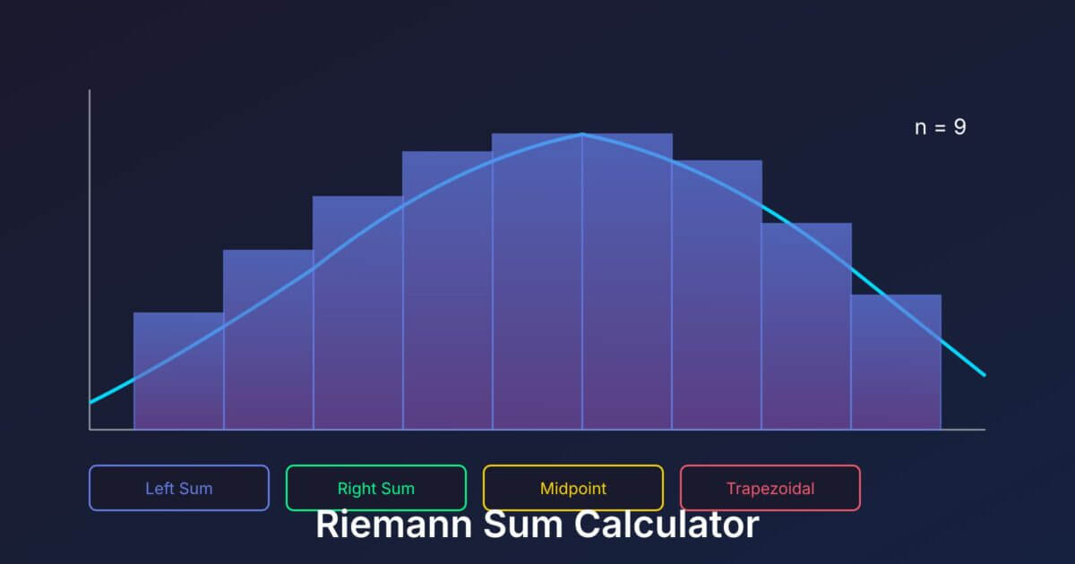
Use this free Riemann Sum Calculator to approximate definite integrals using left, right, midpoint, or trapezoidal sums. Enter your function, set the bounds and number of subdivisions, and see the numerical approximation, error analysis, and an interactive visualization of the rectangles.
Approximate definite integrals using left, right, midpoint, or trapezoidal sums.
Approximation
Visualization
Calculation Details
What is a Riemann Sum?

A Riemann sum approximates the area under a curve by dividing it into rectangles and adding up their areas. Named after German mathematician Bernhard Riemann, this concept forms the foundation of integral calculus.
As the number of rectangles increases (and their width decreases), the approximation gets closer to the exact area, which is the definite integral.
Approximation Methods
Left Riemann Sum
Uses the left endpoint of each subinterval to determine rectangle height. Tends to underestimate for increasing functions, overestimate for decreasing functions.
Right Riemann Sum
Uses the right endpoint of each subinterval. Opposite bias to left sum: overestimates increasing functions, underestimates decreasing functions.
Midpoint Rule
Uses the midpoint of each subinterval. Generally more accurate than left or right sums because errors tend to cancel out.
Trapezoidal Rule
Connects endpoints with straight lines, forming trapezoids instead of rectangles. Often more accurate, especially for smooth functions.
The Formula
For \( n \) rectangles on interval \( [a, b] \):
$$\Delta x = \frac{b – a}{n}$$
$$\sum_{i=1}^{n} f(x_i) \cdot \Delta x$$
where \( x_i \) depends on the method (left, right, or midpoint).
From Riemann Sums to Integrals
$$\int_a^b f(x)\,dx = \lim_{n \to \infty} \sum_{i=1}^{n} f(x_i) \Delta x$$
The definite integral is defined as the limit of Riemann sums as the number of subdivisions approaches infinity. This calculator shows you how the approximation improves as you increase \( n \).
Accuracy Comparison
| Method | Error Order | Notes |
|---|---|---|
| Left/Right | \( O(1/n) \) | Slowest convergence |
| Trapezoidal | \( O(1/n^2) \) | Good for smooth functions |
| Midpoint | \( O(1/n^2) \) | Often best simple method |
Practical Applications
- Numerical integration when antiderivatives are hard to find
- Data analysis when you have discrete measurements
- Physics for calculating work, displacement, or accumulated quantities
- Computer graphics for rendering curves and surfaces
From rectangles to a definite integral
A Riemann sum divides an interval into subintervals, samples the function in each one, and adds rectangle areas. Left, right, and midpoint rules differ only in where that sample point is chosen.
For equal widths, \(\Delta x=(b-a)/n\). Every term must use the same width and an x-value inside its assigned subinterval. Increasing n should usually stabilize the estimate for a well-behaved function.
Compare left and right sums when the function is monotonic. For an increasing positive function, the left sum underestimates and the right sum overestimates. The midpoint rule is often more accurate for the same n.
The result is signed accumulation. Rectangles below the x-axis contribute negatively. If the question asks for total geometric area, split at the zeros and add absolute areas instead.
For \(f(x)=x^2\) on [0, 2] with four equal subintervals, \(\Delta x=0.5\). The left endpoints are 0, 0.5, 1, and 1.5; the right endpoints are 0.5, 1, 1.5, and 2. Writing these points before evaluating prevents an off-by-one rectangle.
The exact integral is \(8/3\), about 2.667. Left and right estimates should bracket that value because \(x^2\) is increasing on this interval. If both estimates land on the same wrong side, recheck endpoints and width.
For unequal subintervals, each rectangle has its own width. Do not apply the equal-width shortcut. The general sum is \(\sum f(x_i^*)\Delta x_i\), and the definite integral is the limit as the largest subinterval width approaches zero.
Common mistakes to avoid
- Using n as the rectangle width
- Sampling outside the correct subinterval
- Expecting exact equality from a small number of rectangles
- Confusing signed integral with total area
Useful calculus books and tools
For Riemann sums, draw the rectangles and distinguish left, right, midpoint, and trapezoidal estimates. Calculus answers are easier to trust when you can connect the symbolic work to a graph, an estimate, and the theorem behind the method.
- Practice beyond one example: Browse calculus textbooks and workbooks on Amazon. Look for worked problems, review exercises, and clear treatment of limits and applications.
- Sketch before calculating: Browse graph-paper notebooks on Amazon. A quick graph often reveals sign errors, incorrect bounds, and unreasonable answers.
As an Amazon Associate, I earn from qualifying purchases.
FAQs
What is the difference between left and right Riemann sums?
Left sums use the function value at the left endpoint of each subinterval for rectangle height; right sums use the right endpoint. For increasing functions, left sums underestimate (rectangles below curve) and right sums overestimate. For decreasing functions, it’s opposite. Neither is inherently better—they have opposite biases.
Why is the midpoint rule more accurate than left or right sums?
The midpoint rule samples the function at the center of each interval, where the rectangle height better represents the average value. Errors above and below the curve tend to cancel out. Mathematically, the midpoint rule has error proportional to 1/n², while left/right have error proportional to 1/n—so midpoint converges much faster.
How many rectangles do I need for an accurate approximation?
It depends on the function and desired accuracy. For smooth functions, 10-20 rectangles often give reasonable estimates. For oscillating or rapidly changing functions, you need more. Watch how the approximation changes as you increase n—when it stabilizes, you’ve reached sufficient accuracy. Trapezoidal and midpoint methods need fewer rectangles than left/right.
How does a Riemann sum become a definite integral?
The definite integral is defined as the limit of Riemann sums as the number of subdivisions approaches infinity: ∫f(x)dx = lim(n→∞) Σf(xᵢ)Δx. As rectangles get infinitely thin, the approximation becomes exact. This limit exists for any continuous function, giving us the precise area under the curve.
What is the trapezoidal rule?
The trapezoidal rule connects the function values at endpoints with straight lines, creating trapezoids instead of rectangles. The area of each trapezoid is ½(f(left) + f(right))·Δx. This is equivalent to averaging left and right Riemann sums. It has O(1/n²) error, making it significantly more accurate than basic Riemann sums for smooth functions.
When would I use Riemann sums instead of antiderivatives?
Use numerical methods when: (1) the antiderivative doesn’t exist in closed form (like e^(-x²)), (2) you only have data points rather than a formula, (3) the function is too complex to integrate symbolically, or (4) you need a quick approximation. Computer calculations routinely use numerical integration—even your calculator uses it internally.
What does the error order O(1/n²) mean?
Error order describes how fast the approximation improves as you add more rectangles. O(1/n) means doubling rectangles cuts error roughly in half. O(1/n²) means doubling rectangles cuts error to about one-quarter. So trapezoidal/midpoint (O(1/n²)) converge much faster than left/right sums (O(1/n)). With 100 rectangles, error is about 100× smaller for O(1/n²) methods.
Can Riemann sums give negative values?
Yes, Riemann sums measure signed area. When the function is below the x-axis, rectangle heights are negative, contributing negative area. The total can be positive, negative, or zero depending on how much area is above vs. below the axis. This signed area concept is fundamental to integration and has physical meaning (like net displacement).