Mean Value Theorem Calculator & Grapher
Here’s the deal: finding the point where a function’s instantaneous rate of change equals its average rate of change is tedious by hand. This mean value theorem calculator does that work for you. It computes the secant slope, checks the MVT hypotheses, locates every point c it can find where the tangent line is parallel to the secant line, and graphs the whole picture.
The tool runs entirely in your browser. Nothing you type is sent anywhere, there is no third-party calculator service behind it, and it works on mobile. Let me show you how it works.
Mean Value Theorem Calculator & Grapher
Enter a function and an interval, then press the button. The calculator does 2 separate jobs: it first verifies that the Mean Value Theorem applies at all, then it finds the guaranteed points. Keeping those jobs separate matters, because the theorem itself only promises that a point exists; locating it is numerical work.
Enter a function and an interval [a, b]. The calculator evaluates the endpoints, computes the secant slope, checks the Mean Value Theorem hypotheses, and locates every point c it can find where the tangent line is parallel to the secant line.
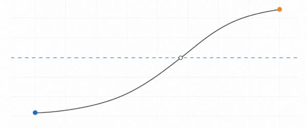
Run the calculator to draw f on [a, b] with the secant line and the tangent lines at each located c.
| x | f(x) | f'(x) |
|---|
The function box accepts standard calculator notation: x^3 – x – 2, sin(x), e^x, sqrt(x), ln(x), abs(x), pi, and implicit multiplication such as 2x or x sin(x). The endpoint boxes take numbers or simple constants like pi/2. Everything runs in your browser; nothing you type is sent anywhere.
The secant states the average. Some tangent must match it.
What is the Mean Value Theorem?
The Mean Value Theorem is one of calculus’s most powerful tools. It tells you something intuitive: if you drive 60 miles in one hour, at some point during that trip, your speedometer must have read exactly 60 mph.
More formally, here’s what MVT guarantees:
If \( f \) is continuous on the closed interval \( [a, b] \) and differentiable on the open interval \( (a, b) \), then there exists at least one point \( c \) in \( (a, b) \) where:
$$f'(c) = \frac{f(b) – f(a)}{b – a}$$
In plain English: somewhere between \( a \) and \( b \), the instantaneous rate of change equals the average rate of change over the entire interval.
The formal statement: If \( f(x) \) is defined and continuous on \( [a, b] \) and differentiable on \( (a, b) \), then there exists at least one number \( c \) in the interval \( (a, b) \) (meaning \( a < c < b \)) such that $$f'(c) = \frac{f(b) – f(a)}{b – a}$$
How to Use the Calculator
I designed this calculator to be straightforward. Here’s the process:
- Enter your function in the \( f(x) \) field using standard calculator notation (use
^for exponents; implicit multiplication such as2xworks). - Set your interval endpoints \( a \) and \( b \). These are the bounds where MVT applies. Numbers and simple constants like
pi/2are both accepted. - Press the button. The calculator evaluates \( f(a) \) and \( f(b) \), computes the secant slope, checks continuity and differentiability, and lists every point \( c \) it locates where \( f'(c) \) equals that slope.
The graph shows your function in dark blue, the secant line connecting the endpoints as a dashed red line, and the tangent line at each located \( c \) in green. Red dots mark the endpoints; green dots mark the tangent points. A table under the graph lists sample values of \( f \) and its derivative across the interval.
Why Use This Calculator?
Let’s be real: you could solve MVT problems by hand. But here’s what this tool gives you:
- Speed: Results in seconds, not minutes of algebraic manipulation.
- Visual understanding: The graph draws the secant line and every located tangent line, so you see why the theorem works, not just that it does.
- Hypotheses first: The calculator checks continuity and differentiability before it claims anything, and it names the problem point when a check fails.
- Multiple solutions: The scan reports every \( c \) it can detect, not just one, with an honest note about what a numerical scan can miss.
- Free and private: Everything runs in your browser. Nothing to install, and nothing you type leaves the page.
For students, teachers, and professionals working through calculus problems, this is a serious time-saver.
Rolle’s Theorem: A Special Case
Here’s the thing: Rolle’s Theorem is just MVT with one extra condition. And once you understand this connection, both theorems click into place.
What if \( f(a) = f(b) \)?
Then the MVT formula simplifies dramatically:
$$f'(c) = \frac{f(b) – f(a)}{b – a} = \frac{0}{b – a} = 0$$
That’s Rolle’s Theorem. If the function starts and ends at the same value, there must be a point where the derivative equals zero: a horizontal tangent.
Rolle’s Theorem (formal): If \( f(x) \) is continuous on \( [a, b] \), differentiable on \( (a, b) \), and \( f(a) = f(b) \), then there exists at least one \( c \) in the open interval \( (a, b) \) (meaning \( a < c < b \)) such that \( f'(c) = 0 \).
Historical note: The Indian mathematician Bhaskara II stated this theorem in the 12th century without formal proof. Michel Rolle provided the rigorous proof in 1691, about 500 years later.
Pro tip: You can use the calculator above for Rolle’s Theorem problems too. Just enter values of \( a \) and \( b \) where \( f(a) = f(b) \), and the calculator will find where \( f'(c) = 0 \). There is also a dedicated Rolle’s theorem calculator when you want the hypotheses stated in Rolle’s own terms.
Don’t confuse this with the Intermediate Value Theorem. That’s a different beast entirely.
MVT vs. Rolle’s Theorem: Quick Comparison
| Feature | Mean Value Theorem | Rolle’s Theorem |
|---|---|---|
| Continuity requirement | Continuous on \( [a, b] \) | Continuous on \( [a, b] \) |
| Differentiability requirement | Differentiable on \( (a, b) \) | Differentiable on \( (a, b) \) |
| Endpoint condition | None | \( f(a) = f(b) \) |
| Conclusion | \( f'(c) = \frac{f(b)-f(a)}{b-a} \) | \( f'(c) = 0 \) |
| Geometric meaning | Tangent parallel to secant | Horizontal tangent exists |
The proof of the Mean Value Theorem
The proof is short once Rolle’s theorem is in hand, and the trick behind it is worth remembering on its own: tilt the picture. Subtract the secant line from \( f \), so that the tilted function starts and ends at the same height, and Rolle’s theorem does the rest.
Define the auxiliary function that measures the vertical gap between the curve and the secant line through \( (a, f(a)) \) and \( (b, f(b)) \):
$$g(x) = f(x) – f(a) – \frac{f(b) – f(a)}{b – a}\,(x – a)$$
The function \( g \) inherits both hypotheses, because it is \( f \) minus a polynomial of degree 1: it is continuous on \( [a, b] \) and differentiable on \( (a, b) \). It also vanishes at both endpoints. At \( x = a \) the gap is \( g(a) = f(a) – f(a) – 0 = 0 \) by construction, and at \( x = b \):
$$g(b) = f(b) – f(a) – \frac{f(b) – f(a)}{b – a}\,(b – a) = 0$$
So \( g \) satisfies every hypothesis of Rolle’s theorem: continuous on the closed interval, differentiable on the open one, equal values at the ends. Rolle’s theorem hands us a point \( c \) in \( (a, b) \) with \( g'(c) = 0 \). Now differentiate \( g \); the secant slope is a constant, so
$$g'(x) = f'(x) – \frac{f(b) – f(a)}{b – a},$$
and setting \( g'(c) = 0 \) gives exactly the conclusion:
$$f'(c) = \frac{f(b) – f(a)}{b – a}$$
That is the whole proof. And the auxiliary function is not a rabbit from a hat: \( g \) is the vertical distance between the curve and its own secant, so the claim “some tangent is parallel to the secant” becomes the claim “the gap function has a flat point”, which is Rolle’s theorem verbatim.
Why Rolle’s theorem itself is true
The chain should not stop at Rolle, because his theorem needs a proof too. It comes from two more basic facts.
- The Extreme Value Theorem: a continuous function on a closed, bounded interval attains a largest and a smallest value. This is where the completeness of the real numbers enters the argument; it is the same foundation the Intermediate Value Theorem stands on.
- Fermat’s interior extremum theorem: if \( f \) has a maximum or minimum at an interior point \( c \) and \( f'(c) \) exists, then \( f'(c) = 0 \). Approaching an interior maximum from the right, the difference quotients \( \frac{f(x) – f(c)}{x – c} \) are at most 0; approaching from the left, they are at least 0. The derivative is the limit of both, so it can only be 0.
Now take \( f \) continuous on \( [a, b] \), differentiable on \( (a, b) \), with \( f(a) = f(b) \). By the Extreme Value Theorem, \( f \) attains its maximum and its minimum somewhere on the interval. If both happen at endpoints, then the maximum equals the minimum, because the endpoint values agree; so \( f \) is constant and \( f'(c) = 0 \) at every interior point. Otherwise at least one extremum sits at an interior point \( c \), and Fermat’s theorem forces \( f'(c) = 0 \) there. Either way, Rolle’s point exists.
The full chain runs from the completeness of the real numbers, through the Extreme Value Theorem and Fermat’s theorem, to Rolle’s theorem, and finally to the MVT. Every link is a few lines long, and nothing in the chain computes anything. That is exactly why the theorem can only promise existence.
What the theorem promises, and what it does not
The Mean Value Theorem promises existence, and existence only. Under its two hypotheses, at least one point \( c \) strictly between \( a \) and \( b \) has its instantaneous rate of change equal to the average rate over the whole interval. Everything else people read into the theorem is not in the statement.
What it promises:
- At least one \( c \) in the open interval \( (a, b) \). Never at an endpoint; the guarantee is strictly interior.
- Exact equality. \( f'(c) = \frac{f(b) – f(a)}{b – a} \) holds exactly, not approximately; the calculator’s decimals are approximations of a point where the identity is perfect.
- Unconditional delivery. Once continuity and differentiability hold, nothing else is needed: no convexity, no monotonicity, not even a formula for \( f \).
What it does not promise:
- Not uniqueness. There can be many valid points; the default example on this page has 2, and \( \sin(x) \) on a long interval has dozens.
- Not location. The theorem never says where \( c \) is, only that it exists. Locating it is numerical work, which is the calculator’s half of the job.
- Nothing when a hypothesis fails. \( f(x) = |x| \) on \( [-1, 1] \) has \( f(-1) = f(1) \), yet no point satisfies \( f'(c) = 0 \): the corner at 0 breaks differentiability, and the promise evaporates with it. The hypotheses are load-bearing, not decoration.
- Nothing about the rest of \( f’ \). The derivative need not be continuous, and the value at \( c \) says nothing about the derivative elsewhere on the interval.
The payoff of even this thin promise is large. If \( f’ = 0 \) across an interval, \( f \) is constant on it. If \( f’ > 0 \), \( f \) is strictly increasing. If two functions share a derivative, they differ by a constant. Each of these is the MVT applied to a subinterval: any two points bracket a \( c \) whose derivative controls the difference of the values. The speeding-camera argument is the same theorem in traffic clothes, and Taylor’s theorem with the Lagrange remainder is the MVT applied repeatedly. One thin existence claim carries a remarkable share of calculus.
Want to go deeper? Check out these 10 Best Selling Real Analysis Books covering the Mean Value Theorem, Rolle’s Theorem, and much more.
Related calculators
When the next step of a problem needs a different theorem, use the Rolle’s theorem calculator, the intermediate value theorem calculator, or the difference quotient calculator. The IVT is the one students mix up with the MVT most: it speaks about function outputs, while the MVT speaks about slopes.
Useful calculus books and tools
For the Mean Value Theorem, verify the hypotheses and compare the secant slope with the derivative at the reported point. Calculus answers are easier to trust when you can connect the symbolic work to a graph, an estimate, and the theorem behind the method.
Calculus: Early Transcendentals by James Stewart
- The differentiation chapters build the Mean Value Theorem and its consequences from the definition up, with worked examples
- Thousands of graded exercises, with answers to odd-numbered problems for self-checking
- The default assigned text in US calculus sequences, so section numbering lines up with most courses
- Formal and heavy; better as a course companion and reference than a first casual read
Calculus: An Intuitive and Physical Approach by Morris Kline
- Teaches through physical meaning first and formal proof second, the right order when a theorem feels arbitrary
- Inexpensive Dover paperback that has stayed in print since 1967
- The best second angle when a standard textbook explanation stalls
- Stops short of a full modern syllabus, so pair it with a course text rather than replacing one
Need more options? See the full list of the best calculus books.
Frequently Asked Questions
What is the Mean Value Theorem used for?
The Mean Value Theorem is used to prove that a function achieves a specific rate of change at some point within an interval. Practical applications include proving speed limits were exceeded (if you traveled 100 miles in 1 hour, you must have hit 100 mph at some point), establishing bounds on function values, and proving other important calculus theorems.
What are the conditions for the Mean Value Theorem to apply?
Two conditions must be met: (1) The function must be continuous on the closed interval [a, b], meaning no breaks or jumps. (2) The function must be differentiable on the open interval (a, b), meaning the derivative exists at every interior point. If either condition fails, MVT may not apply.
How do I find the value of c in the Mean Value Theorem?
First, calculate the average rate of change: (f(b) – f(a))/(b – a). Then find the derivative f'(x) and set it equal to this average. Solve the equation f'(x) = (f(b) – f(a))/(b – a) for x. Any solution in the open interval (a, b) is a valid value of c. Use this calculator to find c values automatically.
What is the difference between Mean Value Theorem and Rolle’s Theorem?
Rolle’s Theorem is a special case of MVT where f(a) = f(b). In this case, the secant line is horizontal, so MVT guarantees a point c where f'(c) = 0. Think of Rolle’s Theorem as MVT with the additional constraint that the function returns to its starting value.
Can there be more than one value of c that satisfies MVT?
Yes, absolutely. The theorem guarantees at least one such c exists, but there can be multiple values. For example, a cubic function on a large interval might have two or three points where the tangent line is parallel to the secant line. This calculator’s scan reports every value it can detect within your interval; values closer together than the scan grid can hide from it.
What happens if the function is not differentiable at a point?
If the function has a corner, cusp, vertical tangent, or discontinuity within (a, b), the Mean Value Theorem does not apply. Common examples include |x| at x = 0 (corner) or x^(1/3) at x = 0 (vertical tangent). Always verify differentiability before applying MVT; this calculator scans for non-smooth points and names the location when it finds one.
How is the Mean Value Theorem related to derivatives?
MVT connects average rate of change (the secant line slope) to instantaneous rate of change (the derivative). It guarantees that somewhere in the interval, these two rates are equal. This relationship is fundamental for proving many derivative properties and is used extensively in differential calculus proofs.
What is the geometric interpretation of the Mean Value Theorem?
Geometrically, MVT says that for any smooth curve connecting two points, there’s at least one place where the tangent line is parallel to the line connecting the endpoints (the secant line). If you draw a line from (a, f(a)) to (b, f(b)), you can always find a point c where the curve has the same slope.
Can I use this calculator for Rolle’s Theorem problems?
Yes! For Rolle’s Theorem, enter any values of a and b where f(a) = f(b). The calculator detects the equal endpoints, notes that you are in the Rolle case, and finds the points c where f'(c) = 0. These are the horizontal tangent points that Rolle’s Theorem guarantees must exist between your chosen endpoints.
How is the Mean Value Theorem proved?
The standard proof subtracts the secant line from f to build the auxiliary function g(x) = f(x) – f(a) – m(x – a), where m is the secant slope. Then g is continuous on [a, b], differentiable on (a, b), and g(a) = g(b) = 0, so Rolle’s theorem gives a point c with g'(c) = 0, which means f'(c) = m. Rolle’s theorem in turn follows from the Extreme Value Theorem and Fermat’s interior extremum theorem, so the whole chain rests on the completeness of the real numbers.
Why does MVT require continuity on a closed interval but differentiability on an open interval?
Continuity at the endpoints a and b is needed to guarantee f(a) and f(b) exist and the function doesn’t jump. However, differentiability at the endpoints isn’t required because we only need a tangent line somewhere in the interior. A function can have corners at a or b and MVT still applies, as long as the interior is smooth.
The habit worth taking from this page: compute the secant slope before you touch the derivative. The slope is the target, the hypotheses are the permission, and the derivative equation is the search. Keep those three steps in that order and most MVT problems reduce to solving one equation.