Maxwell’s Equations

Maxwell’s Equations describe how electric and magnetic fields are produced, how they relate to each other, and how they travel through space. Four short equations encode all of classical electromagnetism — every electric motor, radio antenna, fiber optic cable, MRI scanner, smartphone, and electrical grid in the world operates on the physics they describe. James Clerk Maxwell synthesized them in the 1860s, unifying electricity, magnetism, and light into a single theory.

The deepest result hidden in the equations: a changing electric field creates a magnetic field, and a changing magnetic field creates an electric field. Together they produce self-propagating electromagnetic waves that travel at exactly the speed of light. Maxwell’s prediction that light is an electromagnetic wave was experimentally confirmed by Hertz in 1888 and stands as one of the great unifications in physics.

This study note covers each of the four equations, both their integral and differential forms, the wave equation that follows, the electromagnetic spectrum, applications, the symmetry between fields, common pitfalls, and the historical context that explains why Maxwell ranks alongside Newton and Einstein in the physics pantheon.

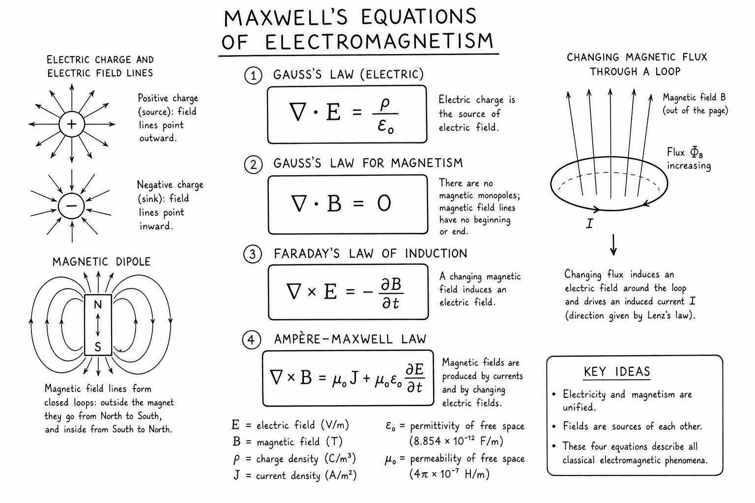
Equation 1: Gauss’s Law

Electric flux through any closed surface equals the enclosed charge divided by \(\varepsilon_0\):

$$\oint \mathbf{E} \cdot d\mathbf{A} = \frac{Q_{\text{enc}}}{\varepsilon_0}$$

In differential form: \(\nabla \cdot \mathbf{E} = \rho / \varepsilon_0\).

This is the field-line picture of electric fields. Field lines emerge from positive charges, terminate on negative charges, and the number of field lines through a surface is proportional to the enclosed charge. Gauss’s law makes computing electric fields with high symmetry (point charges, infinite planes, cylinders, spheres) trivial.

Equation 2: Gauss’s Law for Magnetism

Magnetic flux through any closed surface is always zero:

$$\oint \mathbf{B} \cdot d\mathbf{A} = 0$$

In differential form: \(\nabla \cdot \mathbf{B} = 0\).

This says magnetic monopoles don’t exist — every magnetic field line that enters a closed surface also exits. Cut a bar magnet in half and you get two smaller bar magnets, each with both a north and south pole, never an isolated pole. This asymmetry between electric and magnetic Gauss laws is one of the deep open questions in physics; theoretical extensions like grand unified theories sometimes predict magnetic monopoles but none has been observed.

Equation 3: Faraday’s Law of Induction

A changing magnetic flux induces an electromotive force around a closed loop:

$$\oint \mathbf{E} \cdot d\mathbf{l} = -\frac{d\Phi_B}{dt}$$

In differential form: \(\nabla \times \mathbf{E} = -\partial \mathbf{B} / \partial t\).

This is the principle behind electric generators, transformers, induction motors, and inductive charging. Move a magnet through a coil of wire and you produce a current. The minus sign (Lenz’s law) means the induced current always opposes the change that produced it — a consequence of energy conservation.

Equation 4: Ampère-Maxwell Law

Magnetic fields are produced by electric currents and by changing electric fields:

$$\oint \mathbf{B} \cdot d\mathbf{l} = \mu_0 I_{\text{enc}} + \mu_0 \varepsilon_0 \frac{d\Phi_E}{dt}$$

In differential form: \(\nabla \times \mathbf{B} = \mu_0 \mathbf{J} + \mu_0 \varepsilon_0 \partial \mathbf{E} / \partial t\).

The first term (Ampère’s law) describes the magnetic field around a current-carrying wire — the basis of electromagnets, motors, and solenoids. The second term (Maxwell’s addition) is what makes electromagnetic waves possible: a changing electric field acts like an effective current and produces a magnetic field, even in vacuum where no real charges flow.

The Symmetry Between E and B Fields

The four equations show striking near-symmetry between electric and magnetic fields. Both have a “Gauss law” describing what produces field lines (charges for E, nothing for B). Both have a “curl law” describing how time variation of one field produces the other. The symmetry is broken only by the absence of magnetic monopoles.

This symmetry is exploited in the four-equation summary form using vector calculus. In differential form, Maxwell’s equations can be written even more compactly using differential forms or tensor notation, exposing their relativistic structure: they’re already Lorentz invariant, which is partly why Einstein’s special relativity emerged from electromagnetism rather than from Newton’s mechanics.

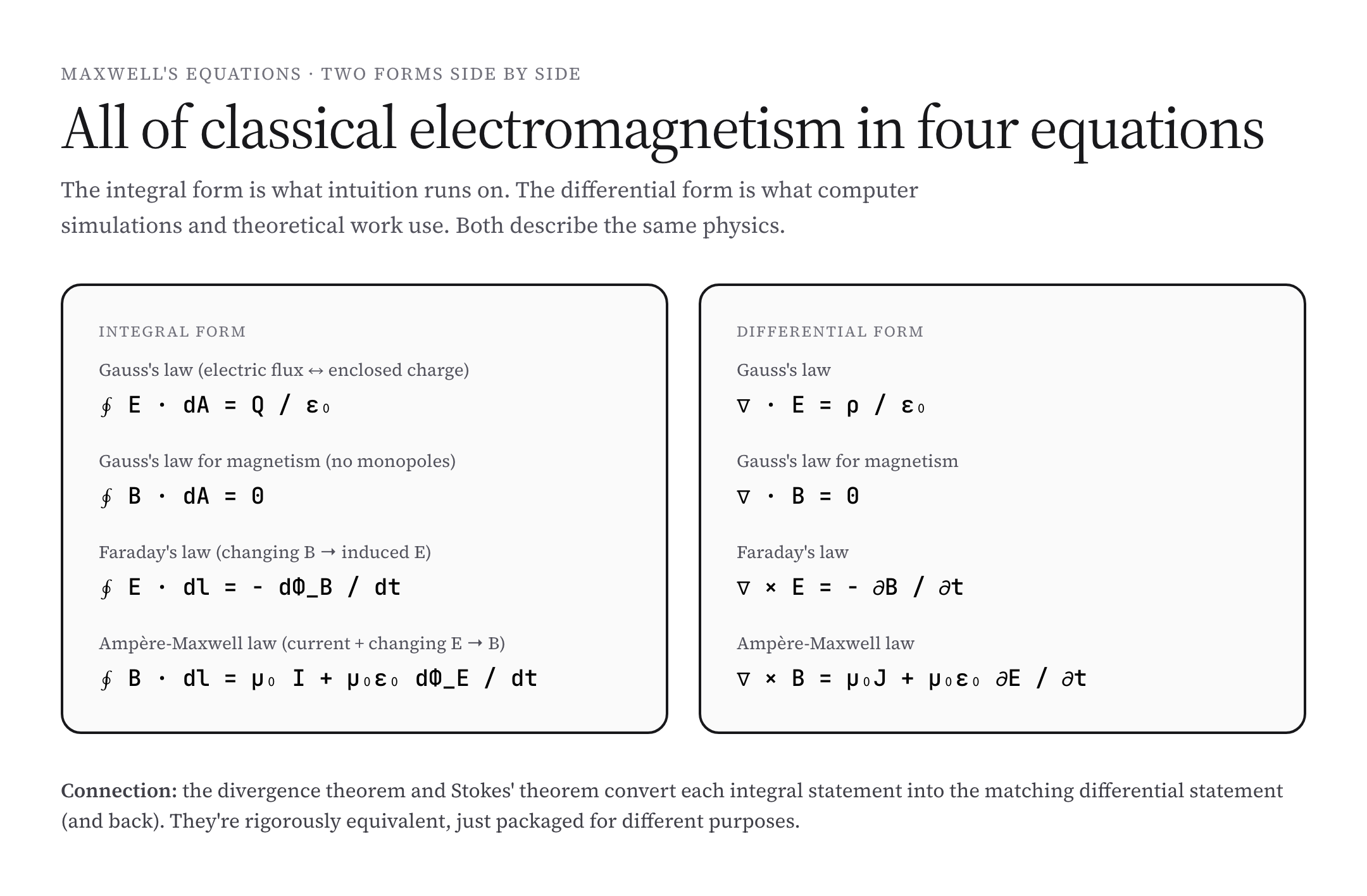
Two Forms: Integral vs Differential

The integral form (left side of each equation as written above) describes total flux or circulation through finite surfaces and around finite loops. It’s what intuition runs on and what you’d use to solve symmetric problems by hand.

The differential form uses divergence and curl operators to describe the same physics at every point in space. Computer simulations, theoretical derivations, and field-equation manipulations all use the differential form. The two forms are connected by Stokes’ theorem and the divergence theorem — they’re rigorously equivalent statements of the same physics.

Deriving the Wave Equation

Combining Faraday’s law and the Ampère-Maxwell law in vacuum (no charges or currents) gives:

$$\nabla^2 \mathbf{E} = \mu_0 \varepsilon_0 \frac{\partial^2 \mathbf{E}}{\partial t^2}$$

This is a wave equation with wave speed \(c = 1/\sqrt{\mu_0 \varepsilon_0}\). Plugging in measured values of \(\mu_0\) and \(\varepsilon_0\) gives \(c = 2.998 \times 10^8\) m/s — exactly the speed of light.

This was Maxwell’s bombshell prediction in 1865: electromagnetic waves exist and travel at the speed of light, so light itself must be an electromagnetic wave. Heinrich Hertz confirmed it experimentally in 1888 by generating and detecting radio waves in the lab. The unification of optics with electromagnetism was one of the most consequential discoveries in physics history.

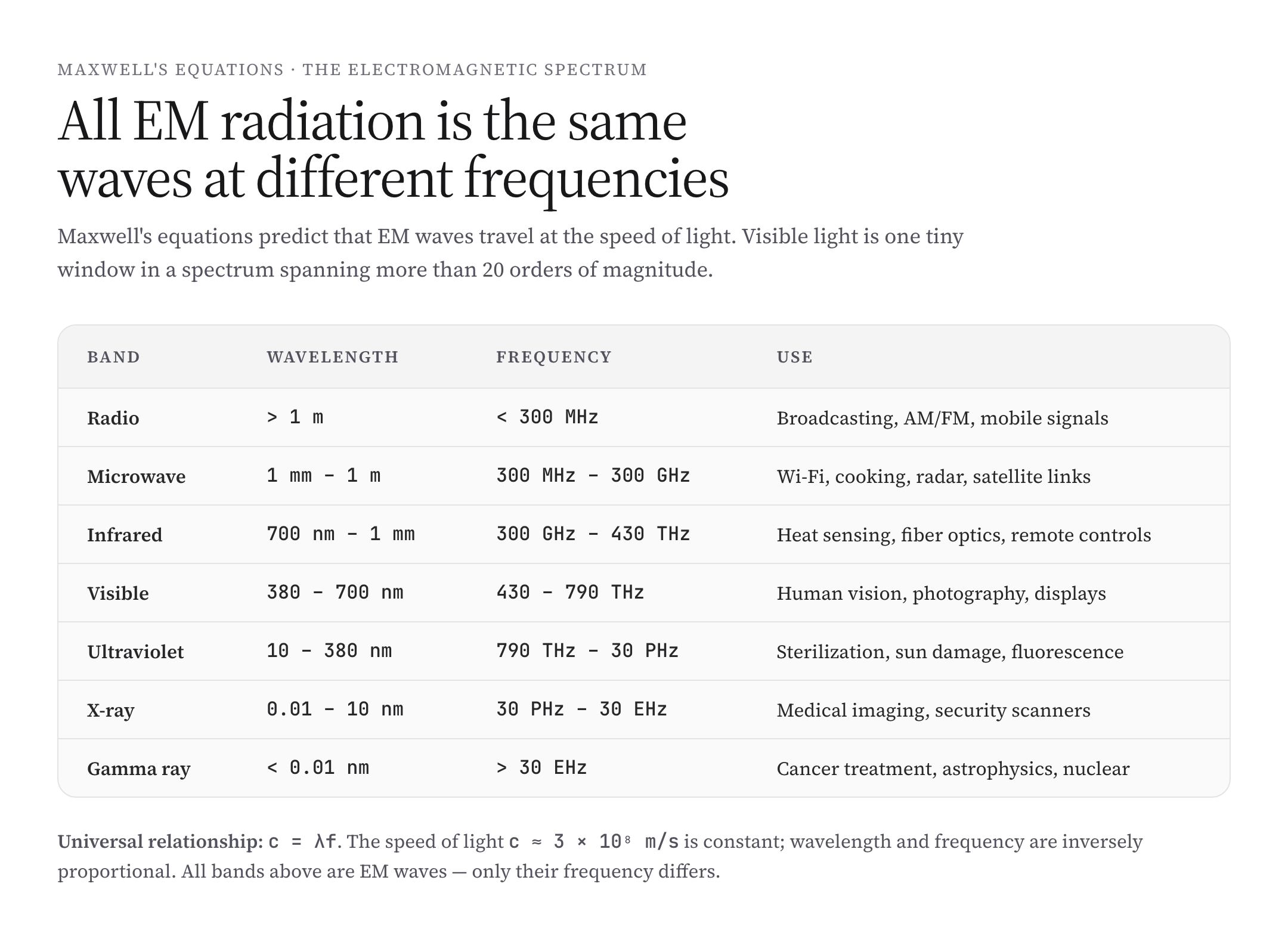
The Electromagnetic Spectrum

EM waves cover an enormous frequency range, from extremely low-frequency radio (long wavelength) through microwaves, infrared, visible light, ultraviolet, X-rays, and gamma rays (extremely short wavelength). All are the same kind of physics — oscillating coupled electric and magnetic fields — at different frequencies.

The relationship is simple: \(c = \lambda f\). Speed equals wavelength times frequency. Visible light occupies a tiny window around 400-700 nm. Below it lies infrared (heat); below that, microwaves (Wi-Fi, cooking) and radio (broadcasting). Above visible light lies ultraviolet (sun damage), then X-rays (medical imaging), then gamma rays (radioactive decay, cosmic sources).

Practical Reference: From Radio to Gamma

Different frequency bands have different uses because their interactions with matter differ. Radio waves pass through walls but bounce off conductive surfaces (radar). Microwaves are absorbed by water (kitchen ovens). Visible light passes through glass and water. UV and X-rays ionize atoms (skin damage, medical diagnostics). Gamma rays penetrate deeply and damage DNA (radiation therapy and radiation hazards).

Engineering applications mirror these properties. Telecommunications uses radio for over-the-horizon broadcast. Wi-Fi and cellular use microwaves for local high-bandwidth links. Fiber optics uses near-infrared for ultra-low-loss long-distance data. Photolithography uses UV for fine semiconductor features. The whole spectrum is the same physics; only the frequency changes its useful applications.

Applications of Maxwell’s Equations

• Power generation and distribution: generators (Faraday’s law), transformers (changing flux induces voltage), AC transmission lines (electromagnetic waves carrying energy).
• Telecommunications: antennas radiate EM waves; receivers detect them. Modulation, demodulation, and signal processing all derive from Maxwell’s equations.
• Optics: lenses, mirrors, fibers, polarization, interference, diffraction — all governed by EM wave propagation in different media.
• Medical imaging: MRI uses radio-frequency electromagnetic waves and magnetic fields. X-ray imaging uses high-energy EM waves. Ultrasound is mechanical, not EM, but EM physics still underlies the transducer electronics.
• Electric motors and actuators: from a watch motor to an EV traction motor, the principle is the Lorentz force on currents in magnetic fields.
• Computers: every transistor, every circuit, every wire carries currents and fields described by Maxwell’s equations. Modern chip design simulates EM behavior at every layer.

Common Mistakes With Maxwell’s Equations

1. Treating E and B as independent. The two fields are coupled by Faraday’s and Ampère-Maxwell laws. Changes in one create the other.
2. Forgetting the displacement current. The \(\partial E/\partial t\) term in Ampère-Maxwell is what makes EM waves possible. Many students remember Ampère’s law without it and get wrong answers in time-varying problems.
3. Mixing up integral and differential forms. They’re equivalent but apply to different geometries. Use integral forms for finite loops/surfaces with high symmetry; use differential forms for point-by-point analysis.
4. Ignoring the minus sign in Faraday’s law. The minus is Lenz’s law — the induced current opposes the flux change. Sign errors here flip the direction of generators and transformers.
5. Confusing static and dynamic cases. Coulomb’s law is the time-independent form of Gauss’s law. Time-varying problems need the full Maxwell apparatus.

A Brief History

Coulomb (1785) studied electrostatic forces; Ørsted (1820) discovered that currents produce magnetic fields; Ampère and Biot-Savart formalized that observation; Faraday (1831) discovered induction. By the 1840s, electricity and magnetism were known to be related but the unification was incomplete.

James Clerk Maxwell synthesized everything in A Dynamical Theory of the Electromagnetic Field (1865), introducing the displacement current term and deriving the wave equation. His original formulation used 20 equations in 20 variables. Oliver Heaviside compressed them into the four-vector form taught today using vector calculus notation.

Hertz’s experimental confirmation (1888) launched radio engineering. Einstein’s special relativity (1905) was directly motivated by trying to reconcile Maxwell’s equations with Newtonian mechanics. By the 1960s, quantum electrodynamics extended Maxwell to the quantum scale, becoming one of the most precisely tested theories in physics history. Maxwell’s classical equations remain accurate for nearly all engineering and most experimental physics.

Modern Significance

Maxwell’s equations underpin essentially every modern electrical and electronic technology. The 19th century invented telegraphy, telephony, and electric power based on early understanding of these laws. The 20th added radio, television, radar, computing, and laser technology. The 21st century is built on optics, photonics, wireless networks, and electromagnetic field manipulation at the nanoscale.

The next century of EM technology — quantum communication, plasmonics, metamaterials, terabit wireless, photonic computing — continues to build on the foundation Maxwell laid down 160 years ago. Few sets of equations have been as productive across as many fields and as many decades as Maxwell’s four.

From Maxwell to Special Relativity

Maxwell’s equations are already Lorentz invariant — they look the same in every inertial frame moving at constant velocity. This contradicted Newton’s mechanics, where the Galilean transformation didn’t preserve the form of the equations. The contradiction was a major puzzle in late 19th century physics.

Einstein’s special relativity (1905) resolved it by modifying mechanics rather than electromagnetism. Time dilation, length contraction, and the relativistic mass-energy relation E = mc² all fall out of requiring physics to be consistent across reference frames moving at constant velocity. Maxwell’s equations stayed unchanged; Newton’s laws were the ones that needed updating. This is one of the most consequential examples in physics of theoretical consistency forcing a deep change in our picture of space and time.

Quantum Electrodynamics

Maxwell’s classical equations are extraordinarily accurate for macroscopic phenomena, but at the atomic scale photons are quantized and the fields fluctuate. Quantum electrodynamics (QED), developed by Feynman, Schwinger, and Tomonaga in the 1940s, replaces Maxwell’s classical fields with quantum field operators.

QED is one of the most precisely tested theories in all of physics. The anomalous magnetic moment of the electron predicted by QED matches experimental measurement to better than one part in a trillion — the highest-precision agreement between theory and experiment ever achieved. For ordinary engineering and most experimental physics, Maxwell’s classical equations remain the working tool; QED takes over only at the quantum level.

How Faraday’s Law Powers Generators

Every electrical generator on Earth runs on Faraday’s law of induction. Spin a coil of wire inside a magnetic field, and the changing flux through the coil induces an EMF that drives current through the external circuit. Hydroelectric, gas, coal, nuclear, wind, and most solar-thermal power plants all use this principle: convert mechanical rotation into electrical current via a changing magnetic flux.

The same physics runs in reverse for motors. Drive current through a coil in a magnetic field, and the Lorentz force makes the coil rotate. Generators and motors are essentially the same machine operated forward and backward — both manifestations of Faraday’s and Ampère’s laws working together. Modern variable-frequency drives, regenerative braking in electric vehicles, and induction cooktops all build on this 200-year-old discovery.

Worked Example: Field of an Infinite Wire

Use Ampère’s law to find the magnetic field around an infinitely long, straight wire carrying current I. Choose a circular Amperian loop of radius r centered on the wire. By symmetry, B is constant in magnitude around the loop and tangent to it.

$$\oint \mathbf{B} \cdot d\mathbf{l} = B \cdot 2\pi r = \mu_0 I$$

Solving: \(B = \mu_0 I / (2\pi r)\). The field circles the wire and falls off as 1/r. This is the textbook example of using Ampère’s law’s integral form to compute a field with high symmetry — far easier than starting from the differential form.

The same approach works for solenoids, toroids, and infinite planes of current. Pick the right symmetry and Maxwell’s integral equations become one-line solutions; without symmetry, you fall back on numerical methods or differential-form analysis.

Conservation of Charge from Maxwell’s Equations

Take the divergence of the Ampère-Maxwell law: \(\nabla \cdot (\nabla \times \mathbf{B}) = 0\) (curl identity), so \(0 = \mu_0 \nabla \cdot \mathbf{J} + \mu_0 \varepsilon_0 \partial(\nabla \cdot \mathbf{E})/\partial t\). Substituting Gauss’s law: \(\nabla \cdot \mathbf{J} + \partial \rho / \partial t = 0\). This is the continuity equation — local conservation of electric charge — derived directly from Maxwell’s equations.

This is the kind of consistency that made Maxwell’s equations so successful: they not only describe the dynamics of E and B fields, they automatically enforce conservation laws that experiment had previously shown to hold. The displacement current term Maxwell added was specifically what made charge conservation come out automatically.

FAQs