Expected Value

Expected value is the probability-weighted average of every possible outcome of a decision. If you repeated the decision a thousand times, expected value tells you what you’d average per attempt. It’s the simplest mathematical tool for thinking under uncertainty, and it beats pure intuition for most everyday choices.

The expected value formula is short, the calculation is fast, and most people who learn it start spotting bad bets they used to take and good bets they used to dismiss. The catch: expected value treats a 50% chance of losing your house the same as a 50% chance of losing a dollar. Survivability matters separately, and any serious decision framework has to layer that consideration on top of raw expected value.

This study note covers the formal definition, several worked examples (project bidding, insurance pricing, gambling), the limitations that ruin people who lean on EV alone, the connection to expected utility, and the everyday mental checklist that turns expected value into a usable thinking tool.

The Formula

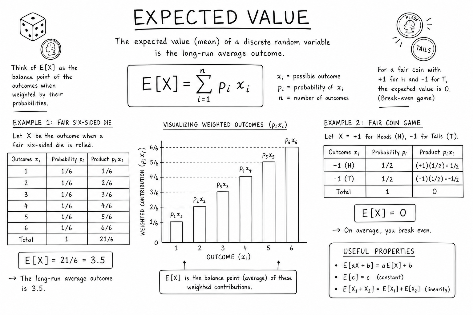
For outcomes \(x_1, x_2, \ldots, x_n\) with probabilities \(p_1, p_2, \ldots, p_n\):

$$E[X] = \sum_{i=1}^{n} p_i \cdot x_i = p_1 x_1 + p_2 x_2 + \ldots + p_n x_n$$

The probabilities must sum to 1. The outcomes can be money, time, units sold, customers retained, lives saved — anything you can put a number on.

For a continuous random variable with probability density function \(f(x)\):

$$E[X] = \int_{-\infty}^{\infty} x \cdot f(x)\, dx$$

The integral version is the same idea expressed for the continuous case. Most everyday decisions live in the discrete world; the integral version becomes essential in finance, physics, and statistics where outcomes vary smoothly.

Worked Example: A Project Bid

You spend 5,000 dollars to prepare a bid. Win the contract (40% chance) and you net 30,000 dollars in profit. Lose the bid (60% chance) and you lose the 5,000 dollars in prep cost.

$$E[\text{bid}] = 0.4 \times 30{,}000 + 0.6 \times (-5{,}000)$$ $$E[\text{bid}] = 12{,}000 – 3{,}000 = 9{,}000$$

Positive expected value. If you face many similar bids over a year, you average 9,000 dollars per attempt. The math says bid.

The deeper insight: expected value also tells you the maximum you should rationally spend on a bid prep. If preparing this bid took 14,000 dollars instead of 5,000, the EV would flip negative (\(0.4 \times 16{,}000 + 0.6 \times (-14{,}000) = 6{,}400 – 8{,}400 = -2{,}000\)) and the math says walk away. Expected value isn’t just a yes/no signal; it’s a calibration for how much resource is worth committing.

Worked Example: An Insurance Premium

Insurance pricing is expected value made visible. A 500,000 dollar policy covers a 0.2% annual risk:

$$E[\text{payout}] = 0.002 \times 500{,}000 = 1{,}000$$

The actuarially fair premium is 1,000 dollars per year. Insurers charge more (say 1,500 dollars) to fund overhead, profit, and the cost of capital they hold against catastrophic claim years. You pay because you’re transferring catastrophic risk, not because the bet is mathematically favorable.

This is also why people buy insurance against rare, large losses (house fires, life insurance, liability) but not against frequent, small losses (lost umbrellas, broken phones). The EV math runs against the buyer in both cases, but the variance reduction is worth the premium when the loss could ruin you. Variance reduction is the product you’re actually paying for.

Worked Example: A Casino Roulette Bet

American roulette has 38 pockets: 18 red, 18 black, 2 green (0 and 00). A bet on red pays 1:1. Probability of winning: 18/38 ≈ 0.474.

$$E[\text{bet}] = \frac{18}{38} \times 1 + \frac{20}{38} \times (-1) = -\frac{2}{38} \approx -5.3\%$$

Every dollar bet on red has an expected value of −5.3 cents. Over many spins, the casino’s edge accumulates with statistical certainty. Casino games exist precisely because the house engineered a negative-EV game and the gambler’s variance lets occasional winners exist long enough to feed the long-term losers.

This is also why advantage gambling — card counting in blackjack, poker against weaker opponents, sports betting against soft lines — works only when the player creates a positive EV through skill or information. Expected value is the line between game-of-chance entertainment and a job.

Where Expected Value Quietly Fails

Two games:

• Game A: guaranteed 100,000 dollars.
• Game B: 10% chance of 1,000,000 dollars, 90% chance of 0 dollars.

Both have \(E = 100{,}000\). Most people prefer Game A. You can’t pay rent with expected value. Expected value treats outcomes as interchangeable as long as the average matches. It doesn’t see ruin.

This is why risk assessment pairs expected value with variance, the Kelly Criterion, and utility functions. Expected value alone is the floor of decision math, not the ceiling.

The St. Petersburg Paradox makes the failure stark. Imagine a coin-flip game where you win \(2^n\) dollars if the first heads occurs on flip \(n\). The expected value is infinite (\(\sum 2^n \cdot 2^{-n} = \sum 1 = \infty\)), yet nobody would pay even 100 dollars to play. Expected value alone doesn’t capture what humans actually value. Daniel Bernoulli proposed the resolution in 1738: people optimize expected utility, not expected value, and utility curves flatten as wealth grows.

Expected Utility: The Standard Fix

Expected utility theory replaces raw outcomes \(x_i\) with utility values \(u(x_i)\), then computes \(E[u(X)] = \sum p_i u(x_i)\). A common choice for \(u\) is the natural logarithm:

$$u(W) = \ln(W)$$

The logarithmic utility function captures diminishing marginal value. The first 100,000 dollars matters more than the second 100,000 dollars, which matters more than the third. A risk-averse decision maker maximizes \(E[\ln(W)]\) instead of \(E[W]\).

For Game A vs Game B above, with starting wealth 100,000 dollars: \(u_A = \ln(200{,}000) \approx 12.21\) vs \(u_B = 0.1 \times \ln(1{,}100{,}000) + 0.9 \times \ln(100{,}000) \approx 11.75\). Game A wins on expected utility, matching the intuitive preference.

Expected utility is the formal foundation for risk-adjusted decision making in finance, insurance, and economics. The Kelly Criterion for optimal bet sizing falls out of maximizing logarithmic expected utility.

Variance: The Other Half of the Picture

Two decisions can share the same expected value and have wildly different risk profiles. The dispersion of outcomes — measured by variance and standard deviation — is what separates them.

For two investments with \(E = 10{,}000\), one with \(\sigma = 2{,}000\) and another with \(\sigma = 10{,}000\), the second carries five times the risk for the same expected return. Sharpe ratio formalizes this idea: return per unit of risk. See the companion notes on variance and standard deviation and the normal distribution for the mechanics.

Quick Mental Checklist

1. List every outcome you can think of, including the bad ones.
2. Estimate a probability for each. Make probabilities sum to 1.
3. Multiply each outcome by its probability. Sum the results.
4. Positive E means the bet is favorable on average.
5. Before acting, ask: can I survive the worst single outcome? If not, expected value isn’t enough.
6. If outcomes vary widely, also estimate variance or worst-case downside before committing.

This six-step pass takes two minutes and catches most obviously bad decisions. For high-stakes calls, layer in variance, downside protection, and expected utility.

Where Expected Value Shows Up Beyond Money

• Marketing. Expected revenue per customer = conversion probability × order value. Drives bid caps in paid search and decisions about whether a campaign is worth running.
• Hiring. Expected value of a candidate = probability of strong performance × upside − probability of poor performance × cost of replacement.
• Engineering reliability. Expected downtime = sum of (failure probability × time to recover) across components.
• Healthcare. Expected quality-adjusted life years (QALYs) for a treatment combine survival probability with quality-of-life adjustments.
• Game design. Loot tables, encounter rewards, and matchmaking algorithms are built on expected value calculations to balance progression and challenge.
• Public policy. Cost-benefit analysis is just expected value applied to civic decisions, with all the strengths and limitations that implies.

Expected value’s power is that it scales. The same one-line formula works for a roulette bet, a venture capital portfolio, a vaccine policy, or a recommendation algorithm. The scaling fails only when you forget to ask whether the average outcome is enough — and when one bad draw can end the game.

Expected Value in Marketing and Advertising

Every paid-ads platform — Google Ads, Meta Ads, LinkedIn Ads — bids on the expected value of a click or impression. The auction sets the price you pay; your expected revenue per click sets your maximum bid. Bid above EV and you lose money on every click. Bid too far below and you lose impressions to competitors.

The formula:

$$\text{Max bid per click} = \text{conversion rate} \times \text{average order value} \times \text{margin}$$

For a 3% conversion rate, $80 average order, and 30% margin, the max bid is \(0.03 \times 80 \times 0.3 = 0.72\) dollars. Anything above that and the campaign loses money on average. Smart marketers compute EV per channel, per audience, and per creative, then optimize accordingly.

Expected Value in Venture Capital

VC portfolios are built on expected value with extreme variance. A typical seed-stage portfolio has an expected return of 2–3× the fund, but most individual investments return zero. The EV math depends on a small number of huge winners (10x, 100x, 1000x) carrying the entire fund.

If you invest $1M each in 30 startups, expected outcomes might look like: 18 fail (return 0), 7 return 2x, 3 return 5x, 1 returns 50x, 1 returns 200x. EV per investment ≈ \((0.6 \times 0 + 0.23 \times 2 + 0.1 \times 5 + 0.033 \times 50 + 0.033 \times 200) \approx 9.3\) million. Total fund EV ≈ 280M on $30M deployed. The math works only because of the extreme tail; ignore it and you’d never make seed-stage bets.

Expected Value vs Median Outcome

For symmetric distributions, expected value (mean) and median agree. For skewed distributions, they can be wildly different. Lottery tickets have positive expected value if the jackpot is large enough, but the median outcome is “lose your dollar.” Startup investments have positive expected value, but the median outcome is “lose your money.”

For one-shot decisions, the median often matters more than the mean. For repeated decisions, the mean is what you converge to. Knowing whether you’re playing a one-shot or a repeated game determines which statistic to anchor on.

Expected Value in Insurance Reserves

Insurance companies set aside reserves to cover expected future claims. The reserve is the present value of expected payouts: \(R = \sum_t \frac{E[\text{payout}_t]}{(1+r)^t}\) where \(r\) is the discount rate.

For a life insurance policy, the expected payout depends on mortality tables (probability of death at each age) multiplied by the policy face value, summed over the policyholder’s remaining expected lifetime. Actuarial science is largely the discipline of computing these expected values reliably across portfolios of millions of policies.

Underestimating expected payouts leads to insurer insolvency. Overestimating leads to uncompetitive premiums. Regulators enforce minimum reserve calculations precisely because the expected-value math is what stands between policyholders and the company’s promise to pay.

Expected Value in Game Theory

In games of strategy, expected value is the standard way to evaluate mixed strategies — strategies that randomize between actions. The Nash equilibrium concept relies on each player’s strategy maximizing their own expected payoff given the others’ strategies.

Rock-paper-scissors has a unique Nash equilibrium where each player picks each option with probability 1/3. Any deviation creates a positive-EV exploitation opportunity for the opponent. Game theorists use this kind of EV reasoning to model auctions, negotiations, voting, and competitive market behavior.

Reinforcement learning extends the same idea to sequential decision making. The Bellman equation is essentially an expected-value recursion: the value of a state equals the immediate reward plus the discounted expected value of the next state.

Expected Value of Perfect Information

Decision theorists compute the expected value of perfect information (EVPI) — how much a decision maker should pay to eliminate all uncertainty before deciding. EVPI is the difference between the expected value of the best decision under uncertainty and the expected value of always making the best decision in each scenario.

If perfect knowledge would only marginally improve outcomes, paying for information isn’t worth it. If EVPI is large, investing in research, surveys, or testing pays off. This is the formal basis for whether to commission a market study, run a pilot, or buy data — answer “is the EVPI greater than the cost?”

Common Pitfalls When Using Expected Value

1. Overconfidence in probability estimates. EV is only as good as the probabilities you plug in. Wide confidence intervals on probabilities translate to wider confidence on EV.
2. Ignoring opportunity cost. A bet with positive EV is still a bad bet if a better positive-EV alternative is available.
3. Not accounting for transaction costs. Trading commissions, taxes, and time costs all eat into expected value. The headline EV is rarely the realized EV.
4. Treating one-shot decisions as repeated. EV converges over many trials. For a single decision with a heavy downside, the expected value can be misleading even when positive.
5. Mixing time horizons. A “positive EV per day” decision might still bankrupt you if the variance is daily and your bankroll is monthly.

Frequently Asked: How EV Connects to Probability and Variance

Expected value is the first moment of a probability distribution. Variance is the second moment around the mean. Together they describe the location and spread of any random variable. Higher moments (skewness, kurtosis) describe asymmetry and tail-heaviness, but EV and variance are the workhorses for everyday decision making.

The relationship between EV and probability is one-way: probability fully determines EV (via integration or summation), but EV alone doesn’t determine probability. Two distributions with the same mean can have wildly different shapes. That’s why pairing EV with variance, or with the full distribution, gives a much more useful picture than EV alone.

FAQs