The Mathematics of Risk Assessment

Every decision involves risk. Hiring someone, launching a product, investing money, choosing a supplier – each carries uncertainty about outcomes. Most people manage this risk intuitively, based on gut feeling and experience. That works until it doesn’t.

Mathematics offers better tools. Probability theory, expected value calculations, variance analysis, and simulation methods let you quantify risk, compare options objectively, and make decisions that optimize for outcomes you actually want.

This article covers the mathematical frameworks for assessing risk. Not academic theory for its own sake, but practical tools you can apply to business and life decisions.

The Foundation: Probability

Risk assessment starts with probability—the mathematical measure of uncertainty. A probability is a number between 0 and 1, where 0 means impossible and 1 means certain. It can also be represented as percentage and fractional values.

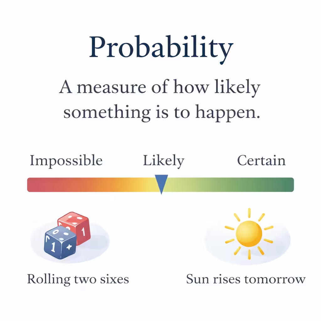
For any event \(A\), we write its probability as \(P(A)\). If you flip a fair coin, \(P(\text{heads}) = 0.5\). If you roll a fair die, \(P(\text{six}) = \frac{1}{6} \approx 0.167\) or 16.7% or just \(\frac{1}{6}\).

Combining Probabilities

When events are independent (one doesn’t affect the other), multiply probabilities:

$$P(A \text{ and } B) = P(A) \times P(B)$$

A 90% reliable system with a 90% reliable backup has:

$$P(\text{both fail}) = 0.1 \times 0.1 = 0.01 = 1\%$$

When events are mutually exclusive (can’t both happen), add probabilities:

$$P(A \text{ or } B) = P(A) + P(B)$$

The probability of rolling a 1 or a 6 on a die:

$$P(\text{1 or 6}) = \frac{1}{6} + \frac{1}{6} = \frac{2}{6} = \frac{1}{3}$$

Complementary Probability

The probability of something not happening is 1 minus the probability it happens:

$$P(\text{not } A) = 1 – P(A)$$

This is often easier to calculate. If there’s a 15% chance of rain, there’s an 85% chance of no rain.

The Problem of Small Probabilities Over Time

A 1% daily failure risk seems small. But over a year?

$$P(\text{at least one failure in 365 days}) = 1 – (0.99)^{365} \approx 0.9747 = 97.47\%$$

That’s why “rare” problems become near-certain over long periods. Small probabilities compound.

Expected Value: The Average Outcome

Expected value (EV) is the probability-weighted average of all possible outcomes. It tells you what you’d get on average if you repeated a decision many times.

For a discrete set of outcomes with values \(x_1, x_2, …, x_n\) and probabilities \(p_1, p_2, …, p_n\):

$$E[X] = \sum_{i=1}^{n} p_i \cdot x_i = p_1 x_1 + p_2 x_2 + … + p_n x_n$$

The Limitation of Expected Value

Expected value treats all outcomes as equally acceptable as long as the average is good. But losing $1 million once hurts more than winning $10,000 one hundred times helps you.

Consider two games:

• Game A: 100% chance of winning $100,000
• Game B: 10% chance of winning $1,000,000, 90% chance of $0

Both have E = $100,000. But most people prefer Game A. You can’t pay rent with expected value.

This leads us to variance.

Variance and Standard Deviation: Measuring Spread

Variance measures how spread out outcomes are around the expected value. Standard deviation is its square root.

$$\text{Var}(X) = E[(X – \mu)^2] = \sum_{i=1}^{n} p_i (x_i – \mu)^2$$

where \(\mu = E[X]\) is the expected value.

$$\text{StdDev}(X) = \sigma = \sqrt{\text{Var}(X)}$$

Comparing Investments

Consider two investments, each requiring $10,000:

Investment A:

• 50% chance: returns $12,000 (+$2,000)
• 50% chance: returns $8,000 (-$2,000)

Investment B:

• 50% chance: returns $20,000 (+$10,000)
• 50% chance: returns $0 (-$10,000)

Both have \(E = \$10{,}000\) (break even on average). But:

For Investment A: $$\sigma_A = \sqrt{0.5 \times (2{,}000)^2 + 0.5 \times (-2{,}000)^2} = \$2{,}000$$

For Investment B: $$\sigma_B = \sqrt{0.5 \times (10{,}000)^2 + 0.5 \times (-10{,}000)^2} = \$10{,}000$$

Investment B has 5× higher standard deviation. Same expected return, five times the risk. Unless you specifically need the possibility of high returns, Investment A is better.

The Coefficient of Variation

To compare risk across different scales, use the coefficient of variation:

$$CV = \frac{\sigma}{\mu}$$

This expresses risk relative to expected return. A 1,000 dollar standard deviation matters more for a 5,000 dollar expected value (CV = 0.2) than for a 100,000 dollar expected value → CV = 0.01.

Risk-Adjusted Return: Sharpe Ratio

The Sharpe ratio measures return per unit of risk:

$$\text{Sharpe Ratio} = \frac{R_p – R_f}{\sigma_p}$$

where:

• \(R_p\) = expected return of the portfolio/investment
• \(R_f\) = risk-free rate (e.g., government bond yield)
• \(\sigma_p\) = standard deviation of returns

Higher Sharpe ratios are better. You’re getting more return for each unit of risk taken.

Example

Investment with 12% expected return, 15% standard deviation, risk-free rate 3%:

$$\text{Sharpe} = \frac{0.12 – 0.03}{0.15} = 0.6$$

Another investment with 18% expected return, 30% standard deviation:

$$\text{Sharpe} = \frac{0.18 – 0.03}{0.30} = 0.5$$

Despite higher expected return, the second investment has lower risk-adjusted return. You’re taking proportionally more risk for the extra gain.

Value at Risk (VaR): Quantifying Downside

Value at Risk answers: “What’s the maximum I can lose with X% confidence?”

If a portfolio has a 95% VaR of $50,000, that means there’s a 5% chance of losing more than $50,000.

For normally distributed returns with mean \(\mu\) and standard deviation \(\sigma\):

$$\text{VaR}{\alpha} = \mu + z{\alpha} \cdot \sigma$$

where \(z_{\alpha}\) is the z-score for confidence level \(\alpha\). For 95% confidence, \(z_{0.05} \approx -1.645\).

Example

A portfolio has daily expected return of 0.04% and daily standard deviation of 1.2%. For a $1,000,000 portfolio, the 95% daily VaR:

$$\text{VaR}{95\%} = 1{,}000{,}000 \times (0.0004 + (-1.645) \times 0.012)$$

$$\text{VaR}{95\%} = 1{,}000{,}000 \times (-0.0193) = -\$19{,}340$$

With 95% confidence, daily losses won’t exceed $19,340. But 5% of the time, they will exceed that.

Limitations of VaR

VaR tells you the threshold but not how bad things can get beyond it. A portfolio might have 95% VaR of $50,000, but the worst 5% of outcomes might average $200,000 in losses or $2,000,000.

Expected Shortfall (ES), also called Conditional VaR, addresses this by averaging the losses beyond VaR:

$$ES{\alpha} = E[L | L > \text{VaR}{\alpha}]$$

This provides more complete risk information.

The Kelly Criterion: Optimal Bet Sizing

The Kelly Criterion tells you what fraction of your capital to risk on a favorable bet to maximize long-term growth.

For a simple bet with win probability \(p\), loss probability \(q = 1-p\), and odds \(b\) (win \(b\) for every 1 risked):

$$f^* = \frac{bp – q}{b} = \frac{p(b+1) – 1}{b}$$

where \(f^*\) is the optimal fraction of capital to bet.

Example: A Favorable Coin Flip

You can bet on a biased coin: 60% heads, 40% tails. Heads pays 1:1 (double your bet). What fraction to bet?

$$f^* = \frac{(1)(0.6) – 0.4}{1} = \frac{0.6 – 0.4}{1} = 0.2 = 20\%$$

Bet 20% of your bankroll each time to maximize long-term growth rate.

Why This Matters for Business

The Kelly Criterion applies beyond gambling:

Investing: How much of your portfolio in any single stock?

Business ventures: How much capital to allocate to a new product line?

Hiring: How aggressively to hire for an uncertain market expansion?

The key insight: even with positive expected value, betting too much is dangerous. Over-betting leads to ruin even with favorable odds.

Fractional Kelly

Most practitioners use “fractional Kelly”—betting some percentage of the Kelly amount (e.g., half-Kelly = 10% in the example above). This reduces variance and risk of ruin at the cost of somewhat lower expected growth.

Bayesian Updating: Revising Probabilities with Evidence

Often you don’t know true probabilities. Bayes’ Theorem lets you update estimates as you gather evidence.

$$P(H|E) = \frac{P(E|H) \cdot P(H)}{P(E)}$$

where:

• \(P(H|E)\) = posterior probability of hypothesis given evidence
• \(P(E|H)\) = likelihood of evidence given hypothesis
• \(P(H)\) = prior probability of hypothesis
• \(P(E)\) = probability of evidence (normalizing constant)

Example: Is This Employee a Good Hire?

You estimate a 70% prior probability that a new hire is a “good performer.” After one month, their output is below average—something that happens with 20% of good performers but 80% of poor performers.

Let \(G\) = good performer, \(B\) = below average first month.

$$P(G|B) = \frac{P(B|G) \cdot P(G)}{P(B)}$$

$$P(B) = P(B|G)P(G) + P(B|\text{not }G)P(\text{not }G)$$ $$P(B) = (0.20)(0.70) + (0.80)(0.30) = 0.14 + 0.24 = 0.38$$

$$P(G|B) = \frac{(0.20)(0.70)}{0.38} = \frac{0.14}{0.38} \approx 0.368$$

Your estimate drops from 70% to about 37%. One data point significantly shifts probability when it’s diagnostic.

The Base Rate Fallacy

Bayes’ Theorem highlights why base rates matter. A 99% accurate test still produces many false positives if the condition is rare.

If a disease affects 0.1% of the population and a test is 99% accurate (99% true positives, 99% true negatives):

$$P(\text{disease}|\text{positive}) = \frac{(0.99)(0.001)}{(0.99)(0.001) + (0.01)(0.999)}$$

$$P(\text{disease}|\text{positive}) = \frac{0.00099}{0.00099 + 0.00999} = \frac{0.00099}{0.01098} \approx 9\%$$

Even with a positive test, there’s only about 9% chance of having the disease. The rare base rate dominates.

Monte Carlo Simulation: When Math Gets Complex

For complicated scenarios with multiple variables and non-obvious distributions, Monte Carlo simulation uses random sampling to estimate outcomes.

The process:

1. Define probability distributions for each uncertain variable
2. Randomly sample from each distribution
3. Calculate the outcome for that scenario
4. Repeat thousands of times
5. Analyze the distribution of outcomes

Example: Project Cost Estimation

A construction project has uncertain costs:

• Materials: $80,000-$120,000 (uniform distribution)
• Labor: mean $150,000, std dev $20,000 (normal distribution)
• Permits: 80% chance of $10,000, 20% chance of $25,000

Running 10,000 simulations might produce:

Percentile	Total Cost
5th	$242,000
25th	$258,000
50th (median)	$272,000
75th	$287,000
95th	$310,000

You now know: 90% confidence interval is $242,000-$310,000. Budget $285,000 for 75% confidence, $310,000 for 95%.

When to Use Monte Carlo

Monte Carlo becomes valuable when:

• Multiple sources of uncertainty interact
• Distributions are complex (not normal)
• Dependencies exist between variables
• Analytical solutions are intractable

Spreadsheets like Excel can run simple Monte Carlo simulations. More complex scenarios use Python, R, or specialized tools.

Risk Matrices: Qualitative Framework

Not all risks have numerical data. Risk matrices combine likelihood and impact qualitatively.

A typical 5×5 matrix:

MATRIX	Negligible	Minor	Moderate	Major	Severe
Almost Certain	Medium	High	High	Extreme	Extreme
Likely	Medium	Medium	High	High	Extreme
Possible	Low	Medium	Medium	High	High
Unlikely	Low	Low	Medium	Medium	High
Rare	Low	Low	Low	Medium	Medium

Risks in “Extreme” cells need immediate mitigation. “High” risks need management plans. “Low” risks can be accepted or monitored.

Quantifying the Matrix

You can add numbers to make the matrix more useful:

Probability scale:

• Almost Certain: >90%
• Likely: 50-90%
• Possible: 10-50%
• Unlikely: 1-10%
• Rare: <1%

Impact scale (example: revenue impact):

• Negligible: <$1,000
• Minor: $1,000-$10,000
• Moderate: $10,000-$100,000
• Major: $100,000-$1,000,000
• Severe: >$1,000,000

Risk score: Multiply probability midpoint by impact midpoint for rough expected loss.

Applying Risk Math to Decisions

Decision Trees

For sequential decisions with uncertainty, decision trees map out paths and calculate expected values.

Example: Product Launch Decision

Launch options:

1. Full launch: costs $500,000
   • 60% probability: success, revenue $2,000,000
   • 40% probability: failure, revenue $200,000
2. Limited launch: costs $100,000
   • 70% probability: success, revenue $400,000
   • 30% probability: failure, revenue $50,000
3. No launch: $0 cost, $0 revenue

Expected value calculations:

Full launch: $$E = 0.6 \times (\$2{,}000{,}000 – \$500{,}000) + 0.4 \times (\$200{,}000 – \$500{,}000)$$ $$E = 0.6 \times \$1{,}500{,}000 + 0.4 \times (-\$300{,}000) = \$900{,}000 – \$120{,}000 = \$780{,}000$$

Limited launch: $$E = 0.7 \times (\$400{,}000 – \$100{,}000) + 0.3 \times (\$50{,}000 – \$100{,}000)$$ $$E = 0.7 \times \$300{,}000 + 0.3 \times (-\$50{,}000) = \$210{,}000 – \$15{,}000 = \$195{,}000$$

Full launch has higher expected value ($780,000 vs $195,000), but also higher variance and potential for significant loss. The choice depends on your risk tolerance.

Expected Utility Theory

People don’t value money linearly. Losing $100,000 hurts more than gaining $100,000 helps. Expected utility theory models this with a utility function.

A common form is logarithmic utility: $$U(W) = \ln(W)$$

where \(W\) is wealth.

Example with logarithmic utility:

Current wealth: $1,000,000 Gamble: 50% chance to win $500,000, 50% chance to lose $500,000

Expected value: $$E[\text{wealth}] = 0.5 \times \$1{,}500{,}000 + 0.5 \times \$500{,}000 = \$1{,}000{,}000$$

Zero expected change in wealth. But expected utility:

$$E[U] = 0.5 \times \ln(1{,}500{,}000) + 0.5 \times \ln(500{,}000)$$ $$E[U] = 0.5 \times 14.22 + 0.5 \times 13.12 = 13.67$$

Current utility: \(\ln(1{,}000{,}000) = 13.82\)

Expected utility of the gamble (13.67) is lower than current utility (13.82). A risk-averse agent should refuse, even though expected value is neutral.

Common Risk Assessment Errors

Ignoring Correlation

Risks that seem independent often aren’t. In 2008, housing markets across the US declined simultaneously, not independently as models assumed. Correlated risks multiply rather than diversify.

If events \(A\) and \(B\) are positively correlated: $$P(A \text{ and } B) > P(A) \times P(B)$$

Models using independence assumptions underestimate joint probability of bad outcomes.

Confusing Low Probability with Zero Probability

A 0.1% annual risk seems negligible. Over 30 years: $$P(\text{at least once}) = 1 – (0.999)^{30} \approx 3\%$$

Still sounds small. But 3% is one in 33. That’s not a freak occurrence.

Overfitting to Recent Data

If the last 20 years were calm, risk models calibrated to that period underestimate true risk. The absence of past crises doesn’t mean crises can’t happen. Fat-tailed distributions mean extreme events are more likely than normal distributions suggest.

Neglecting Tail Risk

Normal distributions underestimate extreme events. Many real phenomena have fat tails—extreme events are more common than Gaussian models predict.

The 2008 financial crisis was a “25-sigma event” by normal distribution standards—literally should never happen in the universe’s history. It happened because returns aren’t normally distributed.

Use t-distributions or explicit tail modeling for phenomena where extremes matter.

Anchoring on Single Point Estimates

Saying “the project will cost $500,000” ignores uncertainty. Saying “the project will cost $400,000 to $600,000 with 80% confidence, with 10% chance of exceeding $750,000” communicates risk properly.

Always present ranges, not single numbers, for uncertain quantities.

Building Your Risk Assessment Practice

Start simple and add sophistication as needed.

Level 1: Basic Expected Value

For any decision, list outcomes, estimate probabilities, calculate expected value:

$$E = \sum p_i \times \text{outcome}_i$$

This beats pure intuition and catches obviously bad decisions.

Level 2: Include Variance

Add standard deviation or range to expected value. Compare options on risk-adjusted basis. Implement rough Sharpe-ratio thinking: how much return per unit of risk?

Level 3: Formal Probability Updates

Track predictions. When new information arrives, use Bayes’ Theorem to update. Keep a record of your probability estimates and calibrate over time.

Level 4: Monte Carlo Simulation

For complex projects or investments, build spreadsheet models with probability distributions. Run simulations to understand range of outcomes. Use percentiles, not averages, for planning.

Level 5: Full Risk Management Framework

Implement risk matrices for qualitative risks. Calculate VaR for financial positions. Apply Kelly Criterion for position sizing. Model correlations between risks.

Most business decisions only need Level 1 or 2. But knowing the full toolkit lets you apply the right tool to each situation.

The Limits of Risk Mathematics

Mathematics helps you think clearly about risk. It doesn’t eliminate uncertainty. Models are simplifications of reality with assumptions that may not hold.

Common limitations:

• Unknown unknowns. You can’t assign probabilities to risks you haven’t imagined.
• Model error. The mathematical structure might not match reality.
• Parameter error. Even with the right model, estimated probabilities might be wrong.
• Human error. People misapply frameworks, ignore uncomfortable results, and overweight recent experience.

Use mathematical risk assessment as one input, not the final word. Combine it with qualitative judgment, scenario planning, and humility about what you don’t know.

The goal isn’t perfect prediction. It’s better decisions than you’d make without the math. On that criterion, risk mathematics delivers.

FAQs

Free Weekly Newsletter

Clarity for people who build things online

Real-world strategies for founders, bloggers, developers, marketers, and educators. No fluff. Just what works.

Subscribe on Substack →

5,000+ readers · Every Friday