Bayes’ Theorem

Bayes’ Theorem tells you how to update what you believe when new evidence arrives. It’s the formal answer to a deceptively simple question: given what I just observed, how should I revise my estimate of what’s true? The result is a single equation that powers spam filters, medical diagnostics, courtroom forensics, search engines, A/B test analysis, and the entire field of Bayesian statistics.

Most people who learn Bayes’ Theorem stop trusting raw test results and start asking the better question — what’s the actual probability, given the base rate? That mental shift is worth more than any individual application. Once you internalize how priors and likelihoods combine, you’ll catch reasoning errors in news articles, business decisions, and scientific claims that the rest of the room misses entirely.

This study note walks through the formula, the intuition, the most common worked examples, the history, the modern uses, and the mistakes that keep tripping up smart people who haven’t seen Bayes’ Theorem laid out cleanly.

The Formula in Plain English

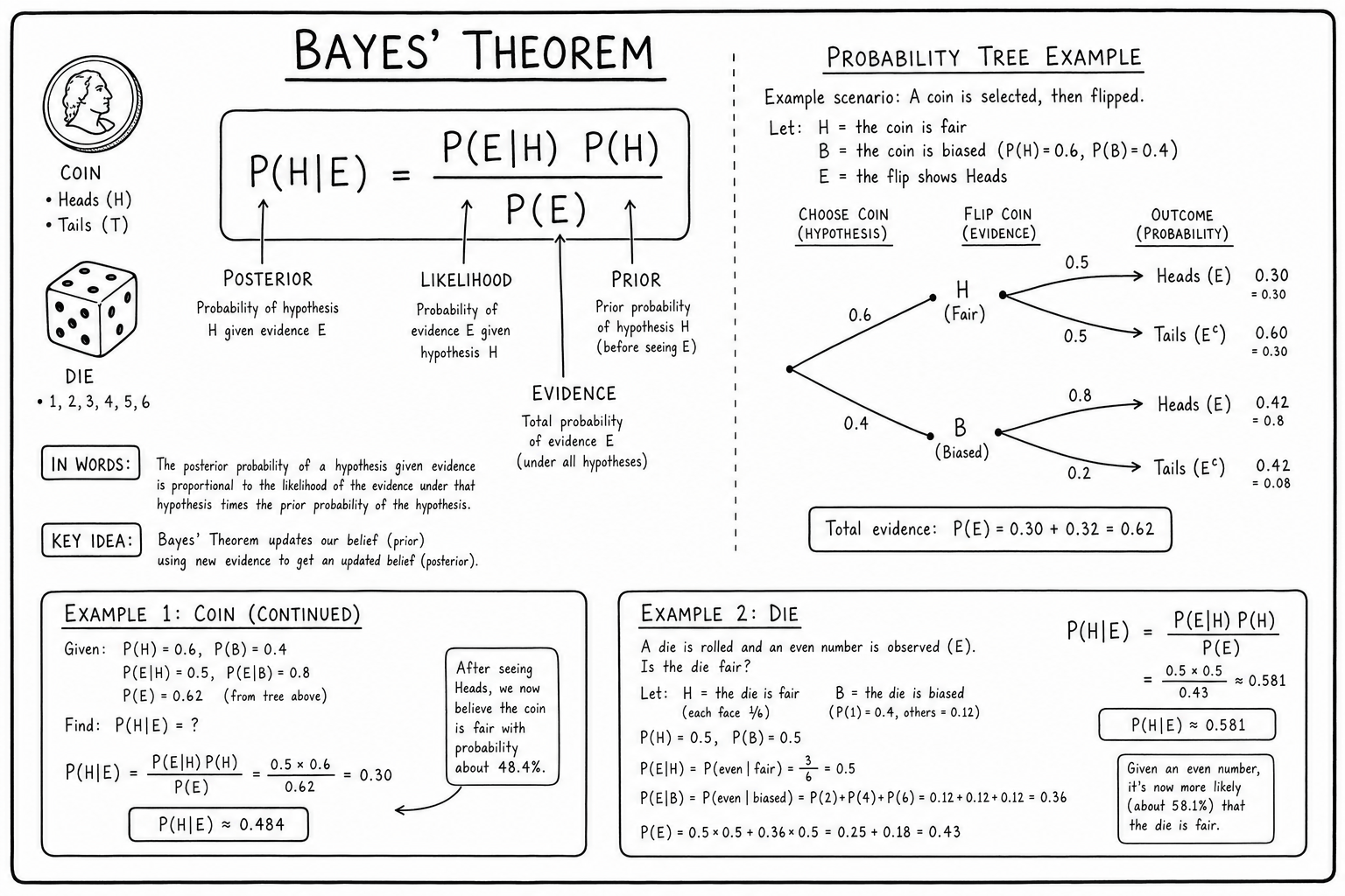
For a hypothesis \(H\) and evidence \(E\):

$$P(H|E) = \frac{P(E|H) \cdot P(H)}{P(E)}$$

Each piece has a name and a job. Memorizing the names makes the formula stop feeling like algebra and start feeling like a recipe.

• \(P(H|E)\) — the posterior. What you want to know after seeing the evidence. The probability the hypothesis is true given the new information.
• \(P(E|H)\) — the likelihood. How likely you’d see this evidence if the hypothesis were true. Often confused with the posterior; they’re not the same.
• \(P(H)\) — the prior. Your probability estimate before seeing the evidence. Usually based on base rates, history, or expert judgment.
• \(P(E)\) — the marginal or evidence. The total probability of seeing the evidence under all hypotheses. Acts as a normalizing constant so the posteriors sum to 1.

The denominator usually expands using the law of total probability:

$$P(E) = P(E|H)P(H) + P(E|\neg H)P(\neg H)$$

That expansion is what turns Bayes’ Theorem from an abstract identity into a calculator-friendly procedure.

Worked Example: A 99% Accurate Test

A disease affects 1 in 1,000 people. A test is 99% accurate, meaning it returns a correct positive 99% of the time and a correct negative 99% of the time. You test positive. What’s the probability you actually have the disease?

The intuitive guess is 99%. The real answer is closer to 9%. Here’s the calculation:

$$P(D|+) = \frac{P(+|D) \cdot P(D)}{P(+|D)P(D) + P(+|\neg D)P(\neg D)}$$ $$P(D|+) = \frac{0.99 \times 0.001}{(0.99)(0.001) + (0.01)(0.999)} = \frac{0.00099}{0.01098} \approx 9\%$$

The base rate dominates. When the condition is rare, even a highly accurate test produces mostly false positives because there are simply more healthy people than sick ones in the testing pool. For every 100,000 people tested with this prevalence: 99 sick people get a positive (true positives) and 999 healthy people get a positive (false positives). Total positives = 1,098. Of those, only 99 actually have the disease — about 9%.

This is the central practical lesson of Bayes’ Theorem. The accuracy of a test alone tells you almost nothing about what a positive result means. You need the prevalence, the false positive rate, and Bayes’ Theorem to put them together.

Worked Example: Spam Filtering

Email spam filters are textbook Bayesian classifiers. The hypothesis: “this email is spam.” The evidence: a particular word like “viagra” appearing in the body.

Suppose 30% of all email is spam (\(P(S) = 0.3\)). Among spam, the word “viagra” appears in 40% of messages (\(P(V|S) = 0.4\)). Among legitimate email, it appears in 0.1% (\(P(V|\neg S) = 0.001\)). What’s the probability an email is spam given it contains “viagra”?

$$P(S|V) = \frac{(0.4)(0.3)}{(0.4)(0.3) + (0.001)(0.7)} = \frac{0.12}{0.1207} \approx 99.4\%$$

Even though only 0.1% of legitimate email contains the word, the strong asymmetry between spam-likelihood and ham-likelihood pushes the posterior to near-certainty. Real spam filters extend this to thousands of features (a “naive Bayes” classifier multiplies the contributions of independent words), but the core math is exactly this.

The Base Rate Fallacy

The base rate fallacy is the habit of ignoring \(P(H)\) and treating the likelihood \(P(E|H)\) as though it were the posterior \(P(H|E)\). People do this constantly:

• “The test is 99% accurate, so I almost certainly have it.” Ignores how rare the condition is.
• “This applicant nailed the interview, so they’re a great hire.” Ignores how often interview-strong candidates underperform on the job.
• “The fraud model flagged this transaction, so it’s probably fraud.” Ignores the volume of legitimate transactions that get false-flagged.
• “This fancy stock-picking newsletter called the last three rallies, so they really know what they’re doing.” Ignores how many newsletter writers exist; some will be lucky three times.

The fix is a one-line discipline: always ask “how common is this underlying condition before any evidence?” That’s your prior. Without it, the math goes wrong, and the conclusion goes wrong with it.

The base rate fallacy is one of the most-replicated findings in cognitive psychology. Daniel Kahneman and Amos Tversky studied it for decades, and it’s one of the central examples in Kahneman’s Thinking, Fast and Slow. Even trained doctors get it wrong on classroom problems involving disease test interpretation, which is why hospitals increasingly publish positive predictive values alongside test sensitivities.

Bayesian Updating in Practice

You don’t always need a calculator to think Bayesian. The mental shortcut: a posterior moves toward the likelihood ratio, weighted by the prior.

• Strong prior + weak evidence = posterior stays close to the prior. New evidence barely moves the needle.
• Weak prior + strong evidence = posterior swings toward the likelihood. The evidence overwhelms the prior.
• Repeated independent evidence compounds — multiply likelihood ratios across observations to update sequentially.

This is how rational people change their minds. Not in one leap, but in calibrated steps as evidence accumulates. Risk assessment uses Bayesian updating to refine probability estimates as projects unfold and reality contradicts (or confirms) the original plan.

The likelihood ratio is the cleanest way to think about evidence strength: \(LR = P(E|H) / P(E|\neg H)\). An LR of 10 means the evidence is 10 times more likely under the hypothesis than under its negation. Multiply LRs across independent observations and your posterior odds update accordingly. This is the backbone of evidence-based medicine, where diagnostic tests are often reported in terms of likelihood ratios precisely because they update naturally with Bayes’ Theorem.

A Brief History

The theorem is named for the Reverend Thomas Bayes, an 18th-century English Presbyterian minister and amateur mathematician. He never published the result during his lifetime. After his death in 1761, his friend Richard Price found the manuscript and submitted it to the Royal Society in 1763.

For nearly two centuries, Bayes’ Theorem was viewed by mainstream statisticians as philosophically dubious because it required prior probabilities, which seemed subjective. The frequentist school led by R.A. Fisher and Jerzy Neyman dominated 20th-century statistics, and Bayesian methods were quietly sidelined.

The Bayesian revival came in the late 20th century for two reasons. First, computers made it possible to run the heavy numerical integration that Bayesian inference often requires (Markov Chain Monte Carlo, or MCMC, became practical in the 1990s). Second, machine learning quietly adopted Bayesian thinking everywhere — naive Bayes classifiers, Bayesian networks, probabilistic programming, variational inference. Today Bayesian methods are mainstream across data science, machine learning, and applied statistics.

Where Bayes’ Theorem Shows Up

• Spam filters. Update probability that a message is spam given the words it contains. Naive Bayes is fast, robust, and surprisingly effective for text classification.
• Medical diagnosis. Combine prevalence, test sensitivity, and test specificity into a real probability of disease. The standard NHS and CDC guidance for interpreting test results uses Bayesian reasoning under the hood.
• A/B testing. Bayesian methods report posterior probabilities of one variant winning rather than p-values. Tools like Optimizely and VWO have embraced Bayesian reporting because it answers the actual business question (“is variant B better?”) instead of the confusing frequentist alternative (“would we see a result this extreme by chance?”).
• Search and recommendation. Update relevance estimates as users click or skip results. This is the basic Bayesian model behind ranking algorithms.
• Insurance and risk pricing. Refine premiums as claims history accumulates. Credibility theory in actuarial science is essentially Bayesian updating of expected loss rates.
• Forensic science. Likelihood ratios for DNA evidence, fingerprints, and document analysis are presented to courts using Bayesian frameworks. The “prosecutor’s fallacy” — confusing \(P(E|innocent)\) with \(P(innocent|E)\) — is a textbook Bayesian error that has overturned wrongful convictions.
• Cybersecurity. Anomaly detection systems compute the posterior probability that a behavior is malicious given an observed pattern. False positive rates that ignore base rates produce alert fatigue and missed real attacks.

Common Mistakes to Avoid

1. Confusing \(P(E|H)\) with \(P(H|E)\). They’re different probabilities. The probability of seeing evidence given a hypothesis is not the same as the probability of the hypothesis given the evidence. This is the classic error behind the prosecutor’s fallacy.
2. Ignoring the base rate. Without \(P(H)\), you can’t compute the posterior. A 99% accurate test on a 0.1% prevalence condition still produces mostly false positives.
3. Assuming independence when it doesn’t hold. Naive Bayes works because it assumes features are conditionally independent. When features are strongly correlated, the math overcounts evidence and the posterior gets pushed to extremes.
4. Picking convenient priors. Priors should reflect honest beliefs before evidence. Cherry-picking a prior to push the posterior in a desired direction is data manipulation, not Bayesian reasoning.
5. Stopping after one update. Bayesian inference is a continuous process. New evidence changes the posterior, and the new posterior becomes the prior for the next round of updating. Treating it as a one-shot calculation misses the point.

Bayesian vs Frequentist: A Quick Note

Frequentist statistics treats probability as long-run frequency of repeated events. Bayesian statistics treats probability as degree of belief that updates with evidence. Bayes’ Theorem itself is a mathematical fact both schools accept; the disagreement is about whether priors are legitimate inputs to inference.

In practice, Bayesian methods give you direct probability statements (“there’s a 73% chance variant B is better”). Frequentist methods give you confidence intervals and p-values, which require careful interpretation and are routinely misread even by trained scientists. Most modern data analysis blends both — Bayesian for direct interpretation, frequentist for calibration and large-sample efficiency.

Bayesian Inference vs One-Shot Updating

One-shot updating treats Bayes’ Theorem as a single calculation: take a prior, multiply by a likelihood, divide by the marginal, get a posterior. Bayesian inference is the broader practice of doing this continuously as data arrives.

In sequential Bayesian inference, today’s posterior becomes tomorrow’s prior. Over many rounds of evidence, the posterior converges to the truth even if the initial prior was imperfect — provided the priors weren’t degenerate (assigning zero probability to the truth) and the evidence is informative. This is why Bayesian methods are robust to mildly bad priors but catastrophic when a prior assigns zero probability to a hypothesis that turns out to be true.

Modern probabilistic programming tools — Stan, PyMC, TensorFlow Probability — automate Bayesian inference for complex models that would be impossible to update by hand. Markov Chain Monte Carlo (MCMC) and variational inference are the two dominant computational engines.

Conjugate Priors

For some prior–likelihood pairs, the posterior comes out in the same family as the prior. These are called conjugate priors, and they make Bayesian updating algebraically clean.

• Beta + Binomial → Beta posterior. Used for click-through rates, conversion rates, A/B test analysis.
• Gamma + Poisson → Gamma posterior. Used for arrival rates, defect counts, customer support tickets.
• Normal + Normal → Normal posterior. Used for measurement noise, sensor fusion, Kalman filters.
• Dirichlet + Multinomial → Dirichlet posterior. Used for topic models, categorical data, document classification.

Before MCMC made arbitrary likelihoods tractable, conjugate priors were the only way to do practical Bayesian work. They’re still useful for fast, interpretable inference and for building intuition about what Bayesian updating does.

Likelihood Ratios in Forensics

Forensic science increasingly reports evidence as likelihood ratios because they update Bayesian posteriors cleanly. A DNA match might have a likelihood ratio of \(10^9\) — meaning the evidence is a billion times more likely if the suspect is the source than if a random person were the source.

The court still needs the prior odds of guilt to compute the posterior. A 1-in-a-billion match doesn’t mean a 1-in-a-billion chance of innocence; it means the odds of guilt have been multiplied by a billion. If the prior odds of guilt were 1-in-10 (e.g., one suspect among 10 plausible candidates), the posterior odds of guilt are about \(10^8\) to 1 — overwhelming, but not the same as the raw 1-in-a-billion figure.

Misreading likelihood ratios as posterior probabilities is the prosecutor’s fallacy. It has overturned wrongful convictions and is now standard material in forensic statistics curricula.

Bayesian Networks

A Bayesian network is a directed acyclic graph where nodes are random variables and edges represent direct probabilistic dependencies. Each node carries a conditional probability distribution given its parents, and the joint distribution factorizes as a product of these conditionals.

Bayesian networks let you encode complex dependency structures and compute conditional probabilities efficiently. Real applications include medical diagnosis (what’s the probability of disease X given symptoms A, B, C, and risk factor D?), gene expression analysis, fault diagnosis in mechanical systems, and risk assessment in safety-critical engineering.

Inference in Bayesian networks uses algorithms like belief propagation, junction tree, or variational message passing. For large networks with continuous variables, MCMC is often the only feasible approach.

FAQs