The Schrödinger Equation

Q: What does the Schrödinger equation describe?

How the quantum state (wavefunction) of a system evolves in time. It's the quantum analogue of Newton's second law: given the initial state and the Hamiltonian (energy operator), it predicts the wavefunction at all later times. Solutions give energy levels, stationary states, and time evolution.

Q: What is the wavefunction?

A complex-valued function ψ(x, t) that contains all information about a quantum system. The squared magnitude |ψ|² is the probability density of finding the particle at position x at time t. The wavefunction is not directly observable — only |ψ|² and quantities derived from ψ are measurable.

Q: What's the difference between time-dependent and time-independent Schrödinger equations?

The time-dependent form iℏ ∂ψ/∂t = Ĥψ describes how wavefunctions evolve in time. The time-independent form Ĥφ = Eφ is an eigenvalue equation that gives stationary states and allowed energies for systems with time-independent Hamiltonians. The time-dependent solution decomposes into stationary states with time-dependent phases.

Q: What is the Hamiltonian?

The energy operator. For a single particle in a potential V(x), Ĥ = −(ℏ²/2m)∇² + V(x). Eigenvalues of Ĥ are the allowed energy levels; eigenfunctions are stationary states. More complex systems have Hamiltonians with additional interaction and spin terms.

Q: Why is the Schrödinger equation complex (involving i)?

Because wavefunctions encode both magnitude and phase information at every point. The phase is essential for interference and superposition. A real-valued formulation cannot capture quantum interference. Maxwell-style real fields don't suffice; you need genuine complex amplitudes.

Q: What is quantum tunneling?

A purely quantum phenomenon where a particle passes through a potential barrier higher than its kinetic energy. Classical mechanics forbids this; the Schrödinger equation predicts an exponentially decaying wavefunction inside the barrier with nonzero amplitude on the other side. Tunneling powers radioactive decay, scanning tunneling microscopes, and stellar fusion.

Q: What does the particle-in-a-box example teach?

It's the simplest quantum system with quantization. Confined particles have discrete energy levels Eₙ ∝ n²; the lowest energy is nonzero (zero-point energy); the wavefunctions have nodes. These features — quantization, zero-point energy, nodal structure — generalize to nearly every quantum system.

Q: Who derived the Schrödinger equation?

Erwin Schrödinger published it in 1926, building on Louis de Broglie's matter-wave hypothesis. Werner Heisenberg had independently developed matrix mechanics in 1925; Schrödinger soon proved the two formulations were equivalent. Max Born (1926) added the probabilistic interpretation of the wavefunction.

Q: What is the Born interpretation?

Max Born's 1926 proposal that |ψ|² is the probability density of finding the particle at a given position. This made quantum mechanics fundamentally probabilistic and was controversial at the time (Einstein rejected it), but it has held up against every experimental test for nearly a century.

Q: Why is there zero-point energy?

It's a direct consequence of Heisenberg's uncertainty principle. A particle with exactly zero kinetic energy would have exactly zero momentum, requiring infinite position uncertainty. Confined particles cannot achieve this, so the lowest-energy state always has nonzero kinetic energy. The harmonic oscillator's E₀ = ½ℏω is the canonical example.

The Schrödinger equation is the central equation of non-relativistic quantum mechanics. It describes how the quantum state of a system — encoded in the wavefunction $\psi$ — evolves in time. Where Newton’s second law plays the central role in classical mechanics, the Schrödinger equation plays the same role in the quantum regime: given the initial state and the forces (now packaged in a Hamiltonian operator), it predicts the future.

Unlike classical mechanics, which gives definite trajectories, quantum mechanics gives probability distributions. The wavefunction $\psi(x, t)$ is complex-valued; its squared magnitude $|\psi|^2$ is the probability density of finding the particle at position $x$ at time $t$. The Schrödinger equation evolves $\psi$ deterministically; the apparent randomness of measurement outcomes comes from the act of observation collapsing the wavefunction to a definite outcome.

This study note covers the time-dependent and time-independent forms, the wavefunction interpretation, common worked examples, the Hamiltonian operator, applications across modern physics, the limits of the theory, common pitfalls, and the historical context.

Schrödinger equation wavefunction modern textbook illustration

The Time-Dependent Form

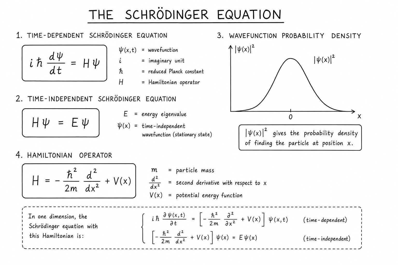
The time-dependent Schrödinger equation:

$$i\hbar \frac{\partial \psi}{\partial t} = \hat{H} \psi$$

Here $\hbar = h / 2\pi \approx 1.055 \times 10^{-34}$ J·s is the reduced Planck constant, $i$ is the imaginary unit, $\psi(x, t)$ is the wavefunction, and $\hat{H}$ is the Hamiltonian operator (which encodes the energy and the forces).

This is a first-order partial differential equation in time. Given the initial wavefunction $\psi(x, 0)$ and the Hamiltonian, you can in principle solve for $\psi(x, t)$ at all later times. The complex $i$ makes $\psi$ inherently complex-valued — quantum mechanics cannot be formulated using only real numbers without losing essential information.

The Time-Independent Form

For systems with time-independent potentials, the wavefunction separates as $\psi(x, t) = \phi(x) e^{-iEt/\hbar}$, and the spatial part satisfies the time-independent Schrödinger equation:

$$\hat{H} \phi = E \phi$$

This is an eigenvalue equation: $\phi$ is the eigenfunction (stationary state), $E$ is the corresponding energy eigenvalue. Solving the time-independent Schrödinger equation gives the allowed energy levels of a system and the corresponding stationary states.

The time-independent form is what students solve in a first quantum mechanics course — the hydrogen atom, particle in a box, harmonic oscillator, and other canonical systems. The full time-dependent solution is built from superpositions of these stationary states with time-dependent phases.

The Wavefunction and Probability Density

The wavefunction $\psi(x, t)$ doesn’t directly give the position of a particle. Instead, $|\psi(x, t)|^2 = \psi^* \psi$ is the probability density of finding the particle at position $x$ at time $t$ when measured. The probability of finding it in an interval is:

$$P(a < x < b) = \int_a^b |\psi(x, t)|^2\, dx$$

For the total probability to be 1, the wavefunction must satisfy $\int |\psi|^2\, dx = 1$ — the normalization condition. Wavefunctions that don’t satisfy this can be normalized by dividing by $\sqrt{\int |\psi|^2\, dx}$.

This probabilistic interpretation (Born, 1926) was one of the most controversial aspects of quantum mechanics. It implies that quantum mechanics is fundamentally probabilistic — there’s no underlying deterministic theory predicting individual measurement outcomes. Einstein famously rejected this (“God does not play dice”), but Born’s interpretation has held up against every experimental test for almost a century.

The Hamiltonian Operator

The Hamiltonian $\hat{H}$ is the energy operator. For a single particle in a potential $V(x)$:

$$\hat{H} = -\frac{\hbar^2}{2m} \nabla^2 + V(x)$$

The first term is the kinetic energy operator (where $\nabla^2$ is the Laplacian). The second is the potential energy. The Hamiltonian’s eigenvalues are the allowed energies of the system; its eigenfunctions are the stationary states.

For more complex systems — multiple particles, electromagnetic interactions, spin — the Hamiltonian gains additional terms. The structure remains the same: kinetic energy plus potential energy plus interaction terms. Modern quantum chemistry and condensed matter physics is largely the practice of writing down the right Hamiltonian for a system of interest and then solving the Schrödinger equation (or approximating it).

Worked Example: Particle in a 1D Infinite Well

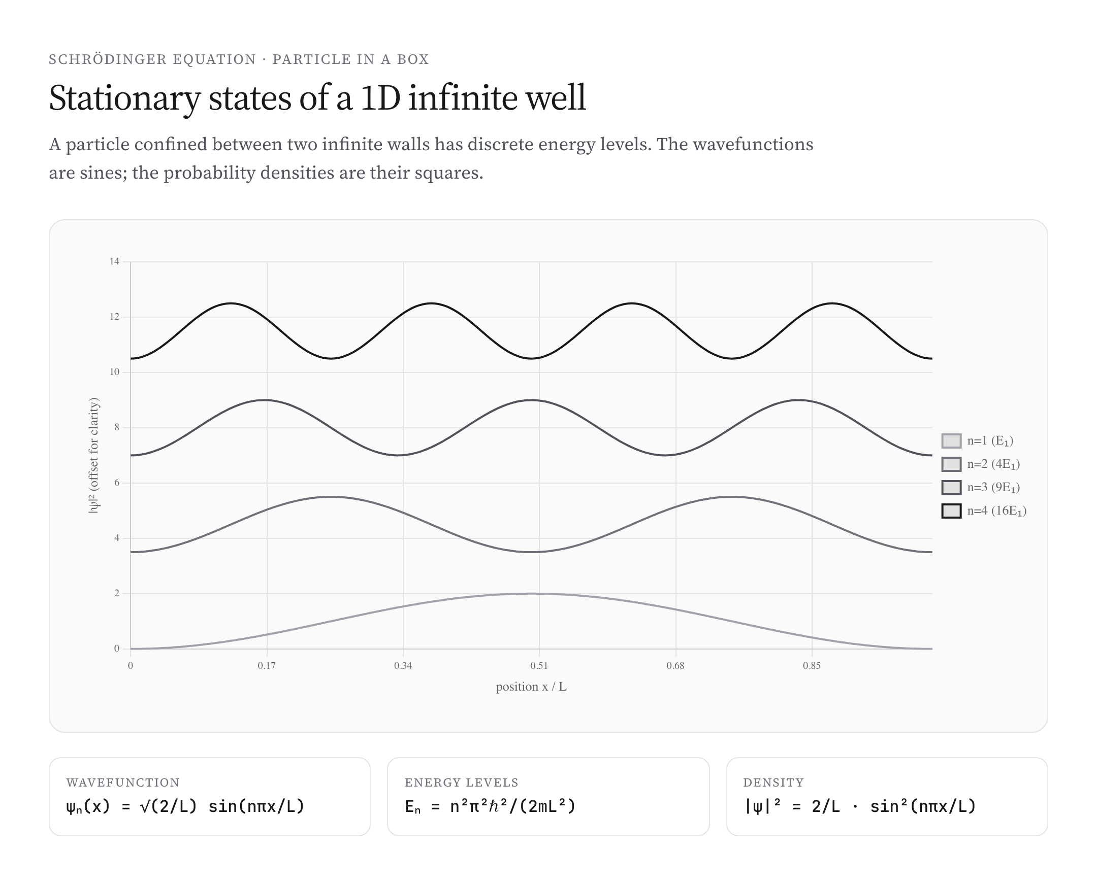
A particle confined to $0 \leq x \leq L$ by infinite potential walls. Inside the well, $V = 0$; outside, $V = \infty$ (so $\psi = 0$). Solving the time-independent Schrödinger equation with boundary conditions:

$$\phi_n(x) = \sqrt{\frac{2}{L}} \sin\left(\frac{n\pi x}{L}\right), \quad E_n = \frac{n^2 \pi^2 \hbar^2}{2mL^2}$$

Energies are quantized — only specific discrete values are allowed, indexed by integer $n = 1, 2, 3, \ldots$. The ground state ($n = 1$) has energy $\pi^2 \hbar^2 / (2mL^2)$, called the zero-point energy. It’s nonzero — the particle can never have exactly zero energy, even at “rest.” This is a direct quantum consequence of Heisenberg uncertainty.

The probability densities $|\phi_n|^2$ have interesting structure: nodes (zeros) at positions where the particle is never found, alternating with high-probability regions. As $n$ grows, the spacing between nodes decreases and the classical limit (uniform probability across the well) emerges.

Worked Example: Quantum Harmonic Oscillator

For $V(x) = \frac{1}{2} m \omega^2 x^2$ (a parabolic potential, like a quantum spring), the Schrödinger equation gives:

$$E_n = \hbar \omega \left(n + \frac{1}{2}\right), \quad n = 0, 1, 2, \ldots$$

Equally spaced energy levels separated by $\hbar \omega$. The ground state energy $\frac{1}{2}\hbar \omega$ is again nonzero (zero-point energy). The wavefunctions are Hermite polynomials times Gaussian envelopes.

The harmonic oscillator is one of the most important model systems in physics because nearly any potential near a minimum is approximately quadratic. Vibrations in molecules, phonons in solids, photons in cavities — all are well-described by quantum harmonic oscillators. The same math reappears constantly across physics.

Stationary state wavefunctions of a particle in a 1D infinite well

Quantum Tunneling

In classical mechanics, a particle with energy $E < V$ cannot enter a region of higher potential. In quantum mechanics, the wavefunction extends into the classically forbidden region with exponentially decaying amplitude. If the barrier is finite in width, the wavefunction emerges with reduced amplitude on the other side — the particle has tunneled through.

The tunneling probability decays exponentially with barrier width and height:

$$T \sim e^{-2\kappa L}, \quad \kappa = \sqrt{2m(V – E)}/\hbar$$

Tunneling underlies radioactive alpha decay, nuclear fusion in stars, scanning tunneling microscopes (atom-by-atom imaging via electron tunneling), and Josephson junctions in superconductors. It’s a purely quantum phenomenon with no classical analogue.

Superposition and Interference

The Schrödinger equation is linear — if $\psi_1$ and $\psi_2$ are both solutions, so is $c_1 \psi_1 + c_2 \psi_2$ for any complex coefficients. This is the principle of superposition: quantum systems can exist in combinations of distinct states simultaneously.

The double-slit experiment is the textbook example. A single electron passes through both slits in superposition; the resulting interference pattern on a screen shows that the electron’s wavefunction interferes with itself. Measuring which slit the electron went through destroys the interference — the act of observation collapses the superposition. This wave-particle duality is at the heart of quantum mechanics.

Quantum Numbers and Atoms

For the hydrogen atom, the Schrödinger equation gives stationary states labeled by four quantum numbers: principal $n$ (energy), angular momentum $\ell$, magnetic $m_\ell$, and spin $m_s$. The energy depends only on $n$: $E_n = -13.6 \text{ eV}/n^2$, reproducing the Rydberg formula for hydrogen spectral lines that had puzzled spectroscopists for decades.

For multi-electron atoms, the Schrödinger equation becomes intractable analytically; numerical methods or approximations (Hartree-Fock, density functional theory) are used instead. The Pauli exclusion principle (no two electrons in the same quantum state) combined with quantum numbers explains the periodic table — element properties recur because outer electron configurations recur.

Where the Schrödinger Equation Lives in Practice

Chemistry: molecular orbital theory, spectroscopy, reaction rates. Quantum chemistry software (Gaussian, ORCA, NWChem) numerically solves the Schrödinger equation for molecules.
Solid state physics: band structure, semiconductors, superconductivity, magnetism. Density functional theory (DFT) is the workhorse computational method.
Particle physics: at low energies, the Schrödinger equation; at relativistic energies, replaced by the Dirac equation and quantum field theory.
Quantum information: qubits, quantum gates, quantum algorithms — all framed in terms of state vector evolution under Hamiltonians.
Materials science: properties of new materials computed from first principles using Schrödinger-equation simulations.
Drug discovery: binding affinities and reaction mechanisms predicted by molecular quantum mechanics.

Limits and Extensions

The Schrödinger equation is non-relativistic. For particles moving near the speed of light, you need the Dirac equation (for spin-1/2 fermions) or the Klein-Gordon equation (for spinless particles). For systems with many interacting particles or quantized fields, quantum field theory takes over.

The Schrödinger equation also doesn’t describe measurement — it evolves states deterministically, while measurement appears to “collapse” the wavefunction probabilistically. The reconciliation between unitary evolution and measurement collapse is the famous quantum measurement problem, and interpretations of quantum mechanics (Copenhagen, many-worlds, decoherence, hidden variables) differ on how to handle it. The math is the same; the philosophy differs.

Common Mistakes

Treating $\psi$ as the particle. The wavefunction is not a physical wave like a water wave. It’s a probability amplitude. $|\psi|^2$ is the probability density.
Forgetting normalization. Wavefunctions must satisfy $\int |\psi|^2 dx = 1$. Unnormalized wavefunctions give incorrect probabilities.
Mixing up the time-dependent and time-independent equations. The time-independent form applies only to stationary states with definite energies. Wavefunctions evolving in time generally aren’t stationary.
Ignoring boundary conditions. The allowed energies and wavefunctions depend critically on boundary conditions (zero at infinity for unbound problems, zero at walls for boxes, smoothness at potential discontinuities).
Confusing classical and quantum analogues. A quantum oscillator has discrete energy levels and zero-point energy; a classical oscillator can have any energy including zero. The math looks similar; the physics differs.

A Brief History

The early 1900s revealed that classical physics couldn’t explain atomic spectra, the photoelectric effect, or blackbody radiation. Planck (1900) introduced energy quanta. Einstein (1905) used quanta for the photoelectric effect. Bohr (1913) proposed quantized electron orbits. De Broglie (1924) suggested matter has wave-like properties.

Erwin Schrödinger published his wave equation in 1926, building on de Broglie’s matter-wave hypothesis. Werner Heisenberg had developed an alternative matrix mechanics formulation in 1925; Schrödinger soon proved the two were equivalent. Max Born (1926) introduced the probabilistic interpretation of the wavefunction.

By 1930, quantum mechanics was largely complete in its non-relativistic form. Paul Dirac extended it to relativistic particles in 1928. Quantum field theory grew through the 1940s-1960s. The Schrödinger equation remains the central equation of non-relativistic quantum mechanics and is taught in every quantum course worldwide.

Solving the Schrödinger Equation Numerically

Most realistic quantum systems can’t be solved analytically. Numerical methods include finite-difference time-domain (discretize space and time), spectral methods (expand in basis functions like sines or Gaussians), and variational methods (minimize energy in a parameter space). The choice depends on the geometry, dimensionality, and boundary conditions of the problem.

Quantum chemistry packages like Gaussian, ORCA, and NWChem use sophisticated combinations of these techniques to solve the many-body Schrödinger equation for molecules with hundreds of electrons. Density functional theory (DFT) is the workhorse for materials science and condensed matter physics, trading exact wavefunction calculations for approximate density-based ones that scale to systems with thousands of atoms.

Identical Particles and Quantum Statistics

For systems of identical particles, the Schrödinger equation requires a symmetry constraint. Bosons (integer spin) have wavefunctions symmetric under particle exchange. Fermions (half-integer spin) have wavefunctions antisymmetric under exchange. The antisymmetry of fermions implies the Pauli exclusion principle: no two fermions can occupy the same quantum state.

This single rule explains the structure of the periodic table (electrons fill atomic orbitals one at a time), the stability of matter (electrons can’t all collapse to the lowest energy state), and white dwarf and neutron star physics (degeneracy pressure preventing gravitational collapse). The connection between spin and statistics — proved by Pauli — is one of the deepest results in quantum mechanics.

Probability Currents and Conservation

The Schrödinger equation implies a continuity equation for probability density: $\partial \rho / \partial t + \nabla \cdot \mathbf{j} = 0$, where $\rho = |\psi|^2$ is the probability density and $\mathbf{j}$ is the probability current density. This is the analogue of charge conservation in electromagnetism — total probability is conserved as the wavefunction evolves in time.

The probability current is what matters in scattering problems and quantum transport. In quantum tunneling through a barrier, the transmitted probability current relative to the incident current gives the transmission coefficient. In semiconductor devices, the same probability-current concept underlies models of electron flow through materials.

Worked Example: Quantum Harmonic Oscillator Energies

The harmonic oscillator V(x) = ½mω²x² is the most important model in physics. Solving the Schrödinger equation gives equally spaced energy levels:

$$E_n = \hbar\omega \left(n + \frac{1}{2}\right), \quad n = 0, 1, 2, \ldots$$

Ground state energy E_0 = ½ℏω is nonzero — the zero-point energy. Successive levels are separated by ℏω. Vibrating molecules, phonons in crystals, photons in cavities, and many other quantum systems all behave like collections of harmonic oscillators in their lowest excitations.

The wavefunctions are Hermite polynomials times Gaussian envelopes, and the system has many remarkable analytical properties — coherent states, ladder operators, classical limits — that make it the canonical pedagogical example of solving the Schrödinger equation.

Hydrogen Atom and Quantum Numbers

The Schrödinger equation for a hydrogen atom in 3D gives stationary states labeled by four quantum numbers: principal n, angular momentum ℓ, magnetic m_ℓ, and spin m_s. The energy depends only on n: E_n = −13.6 eV / n². This reproduces the Rydberg formula for hydrogen spectral lines, which had been measured empirically for decades before quantum mechanics explained it.

For multi-electron atoms, exact analytical solutions don’t exist, but numerical methods (Hartree-Fock, density functional theory) extend the same picture. The Pauli exclusion principle (no two electrons share all quantum numbers) combined with quantum numbers explains the periodic table. Element properties recur because outer electron configurations recur — direct consequence of solving the Schrödinger equation for atoms.

FAQs

What does the Schrödinger equation describe?

How the quantum state (wavefunction) of a system evolves in time. It’s the quantum analogue of Newton’s second law: given the initial state and the Hamiltonian (energy operator), it predicts the wavefunction at all later times. Solutions give energy levels, stationary states, and time evolution.

What is the wavefunction?

A complex-valued function ψ(x, t) that contains all information about a quantum system. The squared magnitude |ψ|² is the probability density of finding the particle at position x at time t. The wavefunction is not directly observable — only |ψ|² and quantities derived from ψ are measurable.

What’s the difference between time-dependent and time-independent Schrödinger equations?

The time-dependent form iℏ ∂ψ/∂t = Ĥψ describes how wavefunctions evolve in time. The time-independent form Ĥφ = Eφ is an eigenvalue equation that gives stationary states and allowed energies for systems with time-independent Hamiltonians. The time-dependent solution decomposes into stationary states with time-dependent phases.

What is the Hamiltonian?

The energy operator. For a single particle in a potential V(x), Ĥ = −(ℏ²/2m)∇² + V(x). Eigenvalues of Ĥ are the allowed energy levels; eigenfunctions are stationary states. More complex systems have Hamiltonians with additional interaction and spin terms.

Why is the Schrödinger equation complex (involving i)?

Because wavefunctions encode both magnitude and phase information at every point. The phase is essential for interference and superposition. A real-valued formulation cannot capture quantum interference. Maxwell-style real fields don’t suffice; you need genuine complex amplitudes.

What is quantum tunneling?

A purely quantum phenomenon where a particle passes through a potential barrier higher than its kinetic energy. Classical mechanics forbids this; the Schrödinger equation predicts an exponentially decaying wavefunction inside the barrier with nonzero amplitude on the other side. Tunneling powers radioactive decay, scanning tunneling microscopes, and stellar fusion.

What does the particle-in-a-box example teach?

It’s the simplest quantum system with quantization. Confined particles have discrete energy levels Eₙ ∝ n²; the lowest energy is nonzero (zero-point energy); the wavefunctions have nodes. These features — quantization, zero-point energy, nodal structure — generalize to nearly every quantum system.

Who derived the Schrödinger equation?

Erwin Schrödinger published it in 1926, building on Louis de Broglie’s matter-wave hypothesis. Werner Heisenberg had independently developed matrix mechanics in 1925; Schrödinger soon proved the two formulations were equivalent. Max Born (1926) added the probabilistic interpretation of the wavefunction.

What is the Born interpretation?

Max Born’s 1926 proposal that |ψ|² is the probability density of finding the particle at a given position. This made quantum mechanics fundamentally probabilistic and was controversial at the time (Einstein rejected it), but it has held up against every experimental test for nearly a century.

Why is there zero-point energy?

It’s a direct consequence of Heisenberg’s uncertainty principle. A particle with exactly zero kinetic energy would have exactly zero momentum, requiring infinite position uncertainty. Confined particles cannot achieve this, so the lowest-energy state always has nonzero kinetic energy. The harmonic oscillator’s E₀ = ½ℏω is the canonical example.

What’s the difference between the Schrödinger equation and quantum field theory?

The Schrödinger equation describes non-relativistic, fixed-particle-number quantum systems. Quantum field theory handles relativistic particles and processes that create or destroy particles (photon emission, particle decay, scattering). For atomic and molecular physics, the Schrödinger equation suffices; for high-energy and particle physics, you need QFT.

What is the measurement problem?

The Schrödinger equation evolves wavefunctions deterministically; measurement appears to collapse them probabilistically to a single outcome. Reconciling these two pictures is the quantum measurement problem. Interpretations differ — Copenhagen says collapse is fundamental; many-worlds says the universe branches; decoherence theories connect the two — but the underlying mathematical formalism is the same.

What is the Pauli exclusion principle?

No two identical fermions (electrons, protons, neutrons) can occupy the same quantum state. Follows from the antisymmetry of fermion wavefunctions under particle exchange. Explains atomic shell structure, the periodic table, the stability of matter, and degeneracy pressure in white dwarfs and neutron stars.

How does the Schrödinger equation handle multiple particles?

By using a multi-particle wavefunction ψ(x₁, x₂, …, xₙ, t) that depends on all particle coordinates. The Hamiltonian includes kinetic energy terms for each particle plus interaction potentials. For identical particles, symmetry constraints (symmetric for bosons, antisymmetric for fermions) apply. Many-body Schrödinger equations are exponentially hard to solve exactly, which is why approximate methods (Hartree-Fock, density functional theory, quantum Monte Carlo) dominate practical computation.