Permutations and Combinations

Permutations and combinations are the two ways to count selections from a set. Permutations count ordered selections — different orderings of the same items count as different. Combinations count unordered selections — different orderings of the same items count as the same. The difference between them is exactly one question: does the order matter?

Both are foundational for probability, statistics, combinatorics, and any field that needs to count discrete arrangements. Card games, password strength, lottery odds, committee selection, route planning, scheduling — they all rely on permutation or combination counting somewhere in the analysis. Once you internalize the order-matters question, every counting problem becomes a one-formula calculation.

This study note covers the formulas, the central distinction, multiple worked examples, the binomial theorem, Pascal’s triangle, applications across probability and computer science, common pitfalls, and a brief history.

The Two Formulas

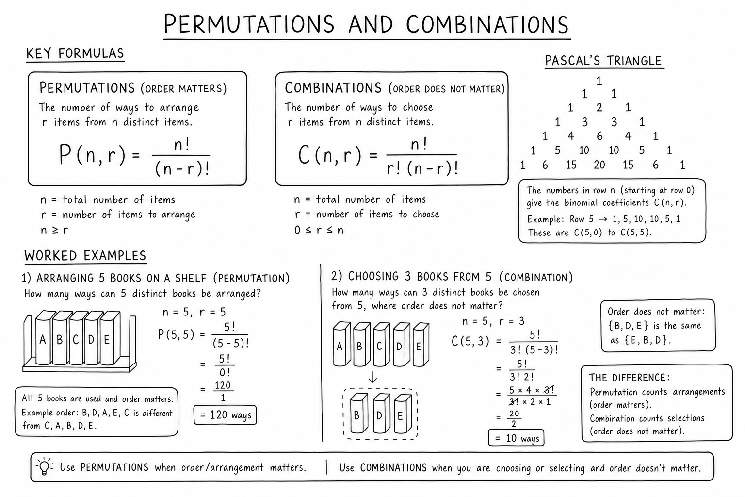
Permutation — order matters:

$$P(n, r) = \frac{n!}{(n – r)!}$$

The number of ways to choose and arrange \(r\) items from \(n\). For \(r = n\) (arranging all of them), this becomes \(n!\).

Combination — order doesn’t matter:

$$C(n, r) = \binom{n}{r} = \frac{n!}{r!(n – r)!}$$

The number of ways to choose \(r\) items from \(n\) without regard to order. Notation: \(\binom{n}{r}\) is read “n choose r.”

The relationship is \(P(n, r) = C(n, r) \cdot r!\) — every combination produces \(r!\) different orderings, so multiplying combinations by \(r!\) gives permutations.

The One Question That Distinguishes Them

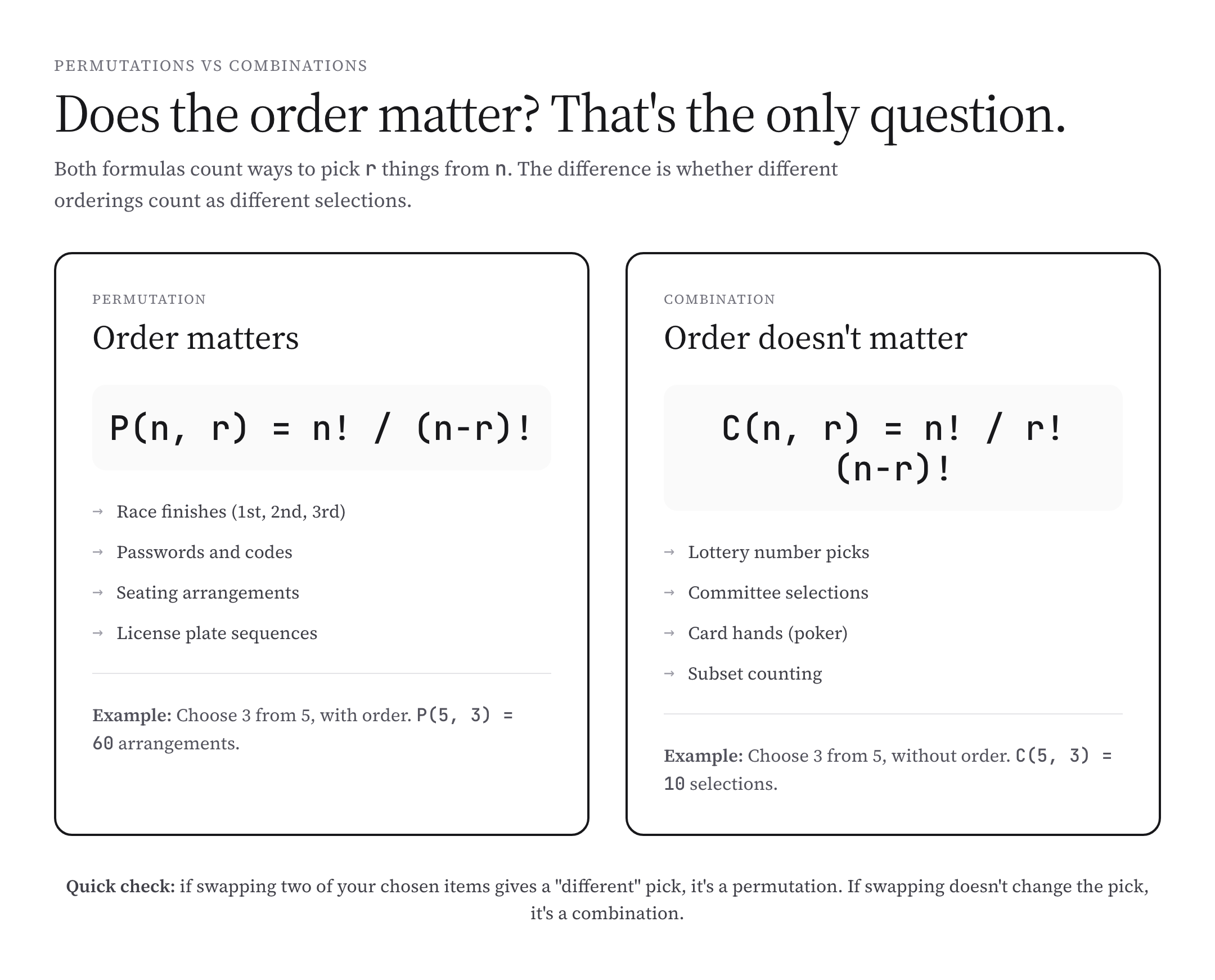
Order matters → permutation. Order doesn’t matter → combination. That’s the entire conceptual difference.

Quick test: pick two items from your selection. Swap them. Does the result count as a different selection?

• Yes (different): permutation. Race finish order, password sequence, license plate.
• No (same): combination. Lottery numbers, poker hand, committee selection.

Almost every counting problem boils down to this one decision. Once you ask “does the order matter?” and answer it correctly, the formula choice is automatic.

Worked Example: A Race

Twelve runners in a race. How many ways can the gold, silver, and bronze medals be distributed?

Order matters (gold ≠ silver ≠ bronze). Permutation:

$$P(12, 3) = \frac{12!}{9!} = 12 \cdot 11 \cdot 10 = 1320$$

1,320 possible podium arrangements. Notice how the formula reduces to the multiplication \(12 \cdot 11 \cdot 10\) — there are 12 choices for first place, 11 for second (one runner already used), 10 for third.

Worked Example: Lottery Numbers

Pick 6 numbers from 1 to 49. How many possible tickets?

Order doesn’t matter (3-7-22-31-38-49 is the same ticket as 49-38-31-22-7-3). Combination:

$$C(49, 6) = \binom{49}{6} = \frac{49!}{6! \cdot 43!} = 13{,}983{,}816$$

Almost 14 million possible tickets. So the chance of winning a 6/49 lottery with one ticket is \(1 / 13{,}983{,}816 \approx 7 \times 10^{-8}\), or about 1 in 14 million. Combinations are how lottery odds get computed.

Pascal’s Triangle and Binomial Coefficients

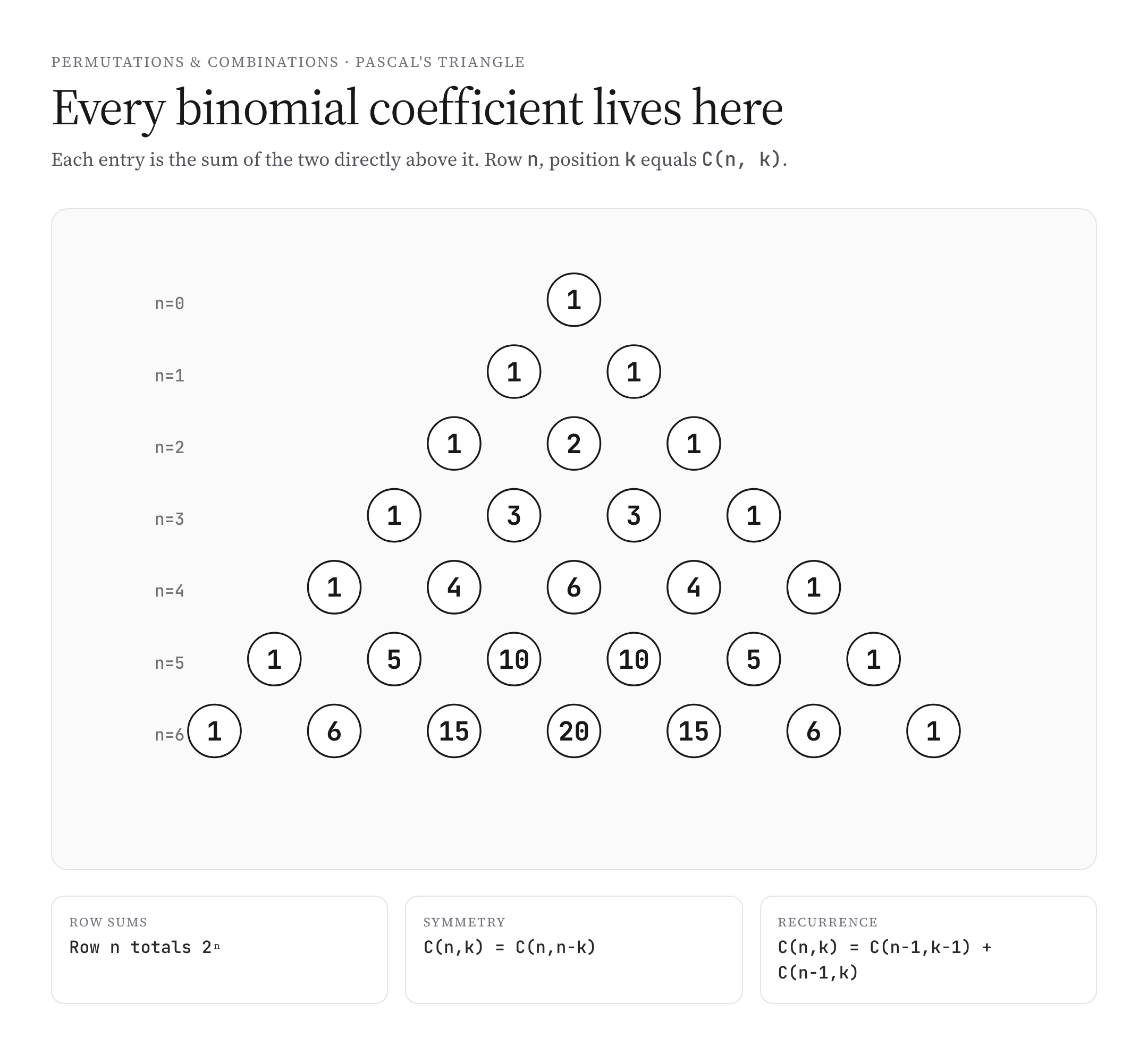
Pascal’s triangle is the array where each entry is the sum of the two directly above it. Row \(n\), position \(k\) (zero-indexed) equals \(\binom{n}{k}\). The first few rows: 1; 1, 1; 1, 2, 1; 1, 3, 3, 1; 1, 4, 6, 4, 1.

The triangle encodes every binomial coefficient up to whatever row you’ve drawn. It’s the cleanest way to look up combinations without computing factorials, especially for small \(n\). It also reveals patterns: row sums equal \(2^n\); entries are symmetric (\(\binom{n}{k} = \binom{n}{n-k}\)); the recurrence \(\binom{n}{k} = \binom{n-1}{k-1} + \binom{n-1}{k}\) is exactly how each entry is built.

The Binomial Theorem

The binomial theorem expands \((a + b)^n\):

$$(a + b)^n = \sum_{k=0}^{n} \binom{n}{k} a^{n-k} b^k$$

The coefficients are exactly the entries in row \(n\) of Pascal’s triangle. So \((a + b)^4 = a^4 + 4a^3b + 6a^2b^2 + 4ab^3 + b^4\) — the row 1, 4, 6, 4, 1 reading left to right.

The binomial theorem is one of the most important identities in algebra. It generalizes to non-integer and negative exponents (the binomial series in calculus) and underlies generating function techniques, power series expansions, and many results in combinatorics and probability.

Worked Example: Coin Flips

Flip a fair coin 10 times. What’s the probability of getting exactly 3 heads?

The number of ways to get 3 heads in 10 flips is \(\binom{10}{3} = 120\). Each specific sequence has probability \((1/2)^{10} = 1/1024\). So:

$$P(\text{3 heads}) = \binom{10}{3} \cdot \frac{1}{1024} = \frac{120}{1024} \approx 11.7\%$$

This is the binomial probability formula. Combinations count the ways to arrange the 3 heads among 10 positions; the probability per arrangement is the same. Multiply, and you have the answer.

Permutations With Repetition

If items can repeat (like in a 4-digit PIN where any digit can repeat), the count is \(n^r\) instead of \(P(n, r)\). For a 4-digit PIN with 10 possible digits per position: \(10^4 = 10{,}000\) possible PINs.

If items don’t repeat (like dealing 5 cards from a deck without replacement), use the standard permutation formula. The replacement vs no-replacement distinction is just as important as the order-matters distinction.

Combinations with repetition (also called multisets) use \(\binom{n + r – 1}{r}\). This counts ways to pick \(r\) items from \(n\) types where types can repeat — the textbook example is choosing scoops of ice cream from a list of flavors where you can pick the same flavor multiple times.

Permutations With Identical Items

Arranging the letters of MISSISSIPPI? It has 11 letters total: 1 M, 4 I’s, 4 S’s, 2 P’s. Identical letters can’t be distinguished, so the count is:

$$\frac{11!}{1! \cdot 4! \cdot 4! \cdot 2!} = 34{,}650$$

The general formula for permutations of multiset elements: \(n! / (n_1! \cdot n_2! \cdots n_k!)\) where \(n_i\) is the count of the \(i\)-th distinct item.

This shows up in DNA sequence counting, anagram problems, scheduling with identical tasks, and any counting problem where some items in the collection are interchangeable.

Where Permutations and Combinations Show Up

• Probability: binomial distributions, hypergeometric distributions, and most combinatorial probability calculations rely on combinations.
• Statistics: sample-space counting for hypothesis tests, exact tests like Fisher’s exact test.
• Cryptography: password strength estimation, key space size, brute-force complexity calculations.
• Computer science: algorithm complexity (the \(\binom{n}{2}\) pairs in pairwise comparisons; subset enumeration; combinatorial optimization).
• Genetics: punnett square outcomes, genotype combinations, probability of inheritance patterns.
• Combinatorial design: tournament schedules, experimental designs, error-correcting codes.
• Game theory and gambling: poker odds, lottery probabilities, blackjack probability calculations.

Common Mistakes With Counting

1. Confusing permutation with combination. The single most common error. Always ask “does the order matter?” before picking the formula.
2. Forgetting whether items can repeat. Permutations with vs without repetition give very different counts. Read the problem carefully.
3. Using the wrong factorial. The denominator in a combination is \(r! (n – r)!\), not just \((n – r)!\). Mixing these up gives permutations instead.
4. Counting the same arrangement twice. When using combinations, ensure you’re not implicitly distinguishing arrangements that should count as the same.
5. Mishandling identical items. Permutations of identical items use the multiset formula, not the standard factorial formula.
6. Off-by-one errors with combinatorial identities. \(\binom{n}{0} = 1\) and \(\binom{n}{n} = 1\), not 0. The empty selection counts.

Useful Identities

• Symmetry: \(\binom{n}{k} = \binom{n}{n-k}\). Choosing what to include is the same as choosing what to exclude.
• Pascal’s recurrence: \(\binom{n}{k} = \binom{n-1}{k-1} + \binom{n-1}{k}\). Either include the first item (then choose \(k-1\) more) or exclude it (choose all \(k\) from the rest).
• Sum of row: \(\sum_{k=0}^{n} \binom{n}{k} = 2^n\). The total number of subsets of an \(n\)-set is \(2^n\), partitioned by subset size.
• Hockey stick identity: \(\sum_{i=r}^{n} \binom{i}{r} = \binom{n+1}{r+1}\). Useful for telescoping combinatorial sums.
• Vandermonde’s identity: \(\binom{m+n}{r} = \sum_k \binom{m}{k}\binom{n}{r-k}\). Used in convolution-style counting.

These identities turn many combinatorial sums into closed-form expressions. They’re worth knowing for both proof writing and competition math.

A Brief History of Combinatorics

Combinatorial counting problems appear in ancient Indian, Chinese, and Greek mathematics. The Indian mathematician Pingala (~300 BCE) studied poetic meters and discovered binomial-coefficient-like patterns. Chinese mathematicians constructed Pascal’s triangle several centuries before Pascal — Yang Hui’s triangle (~1303 CE) is the same array.

Blaise Pascal and Pierre de Fermat formalized combinatorial probability in their 1654 correspondence about gambling problems. Pascal published Traité du triangle arithmétique in 1665, popularizing what’s now Pascal’s triangle in Western mathematics.

Combinatorics flourished in the 19th and 20th centuries through the work of Cayley, Sylvester, MacMahon, Erdős, and many others. Today combinatorics is one of the largest active research areas in mathematics, with deep connections to algebra, geometry, computer science, and probability.

Counting Strategies for Tricky Problems

For complicated counting problems, two strategies dominate.

Inclusion-exclusion principle: count the union of overlapping sets by adding sizes, subtracting pairwise intersections, adding triple intersections, and so on. Used for derangements (permutations with no fixed point), counting integers divisible by various primes, and surveys with overlapping categories.

Complementary counting: count what you don’t want, then subtract from the total. “How many 4-letter words have at least one vowel?” is easier as “Total words minus all-consonant words.” Far easier than directly enumerating cases.

Both strategies turn complex case analyses into straightforward arithmetic. Knowing when to apply each is what separates routine combinatorics from polished problem-solving.

Combinatorics in Computer Science

Combinatorics underpins many algorithm complexity bounds. Sorting requires \(\Omega(n \log n)\) comparisons because there are \(n!\) possible orderings, and each comparison can distinguish at most two of them — so \(\log_2(n!) \approx n \log_2 n\) comparisons are needed in the worst case.

Hash table collision analysis uses combinatorial probability (the birthday paradox). Randomized algorithms use combinatorial bounds to prove correctness with high probability. Cryptographic key-space analysis uses permutation counts to estimate brute-force resistance. Combinatorial reasoning is everywhere in algorithm design.

Stars and Bars (Compositions and Partitions)

“Stars and bars” is a counting technique for distributing identical items into distinct boxes. The number of ways to distribute \(n\) identical items among \(k\) distinct boxes is \(\binom{n + k – 1}{k – 1}\).

Example: how many ways to split 10 identical candies among 4 children? Answer: \(\binom{13}{3} = 286\). The trick is to imagine 10 stars (candies) and 3 bars (dividers) in a row; each arrangement of stars and bars corresponds to a distribution.

Stars and bars also counts the number of non-negative integer solutions to \(x_1 + x_2 + \ldots + x_k = n\), which is the same problem in disguise. It’s the standard technique for any problem involving identical items and distinct categories.

Generating Functions for Counting

Generating functions encode counting sequences as coefficients of polynomials or power series. The coefficient of \(x^n\) in \((1 + x)^k\) is \(\binom{k}{n}\), giving combinations directly.

For more complex problems, generating functions handle constraints elegantly. The number of ways to make change for \(n\) cents using coins of denominations 1, 5, 10, 25 is the coefficient of \(x^n\) in \(\frac{1}{(1 – x)(1 – x^5)(1 – x^{10})(1 – x^{25})}\). Generating functions also generalize to exponential generating functions for permutation-counting problems.

This technique connects combinatorics to power series, calculus, and number theory. It’s a core tool in advanced combinatorial analysis and competitive math.

Worked Example: Counting Without Order, Without Replacement

How many distinct 5-card poker hands are there from a standard 52-card deck? Order doesn’t matter (a hand is the same regardless of dealing order). Replacement doesn’t apply (each card appears once). Combination:

$$C(52, 5) = \binom{52}{5} = \frac{52!}{5! \cdot 47!} = 2{,}598{,}960$$

Just under 2.6 million hands. From this baseline, every poker probability follows: probability of a flush, straight, full house, royal flush — each is a count of favorable hands divided by 2,598,960. Combinatorial counting is the foundation of every poker probability calculation, every blackjack basic-strategy table, and every casino-game expected-value analysis.

Catalan Numbers: A Famous Combinatorial Sequence

The Catalan numbers \(C_n = \binom{2n}{n} / (n+1)\) count many surprising things: the number of valid ways to match \(n\) pairs of parentheses, the number of binary trees with \(n\) nodes, the number of ways to triangulate a convex polygon with \(n + 2\) sides, and the number of monotonic paths along the edges of an \(n \times n\) grid that don’t cross the diagonal.

The first few Catalan numbers are 1, 1, 2, 5, 14, 42, 132, 429. They show up in dozens of seemingly unrelated combinatorial problems and are one of the most fundamental sequences in combinatorics. Recognizing a Catalan number on sight saves enormous derivation work — and it’s a hallmark of strong combinatorial intuition.

Probability Through Counting

For equally likely outcomes, probability equals favorable outcomes divided by total outcomes — both counted via permutations or combinations. The probability of being dealt a flush in poker (5 cards of the same suit) is:

$$P(\text{flush}) = \frac{4 \cdot \binom{13}{5}}{\binom{52}{5}} = \frac{4 \cdot 1287}{2{,}598{,}960} \approx 0.00198$$

About 1 in 500 hands. Numerator: choose a suit (4 ways) and pick 5 cards from that suit. Denominator: total 5-card hands.

Most casino game probabilities, lottery odds, and combinatorial probability problems boil down to this kind of ratio of combinations or permutations. Once you can count both numerator and denominator correctly, the probability follows from one division.

The Birthday Paradox

How many people do you need in a room before two of them probably share a birthday? The intuitive answer (180+) is wildly wrong. The correct answer is just 23.

The math: probability that all 23 birthdays are distinct is \(\frac{365}{365} \cdot \frac{364}{365} \cdot \frac{363}{365} \cdots \frac{343}{365} \approx 0.493\). So the probability of at least one match is about 50.7%.

The birthday paradox is a textbook lesson in combinatorial probability — pairwise comparisons grow as \(\binom{n}{2}\), so with 23 people you have 253 pairs, each with a 1/365 chance of matching. The cumulative probability gets large much faster than intuition suggests. The same math underlies hash collision analysis in cryptography and data structures.

FAQs