Logarithms

Logarithms are the inverse of exponentiation. Where exponents ask “what do I get if I multiply this base by itself \(n\) times?”, logarithms ask “how many times do I have to multiply this base by itself to get this number?” That dual relationship is the entire point of logarithms, and once you internalize it, the algebraic rules and the practical applications fall into place.

Logarithms turn multiplication into addition, division into subtraction, and exponents into multiplication. That’s why they revolutionized computation in the 17th century — slide rules and log tables let scientists multiply huge numbers as fast as they could add them. Today, computers handle the multiplication, but logarithms remain essential for any field that handles quantities ranging across many orders of magnitude (sound, light, earthquakes, computing complexity, finance).

This study note covers the definition, the seven core rules, common bases, the change of base formula, log scales versus linear scales, applications across disciplines, common pitfalls, and a brief history.

Definition

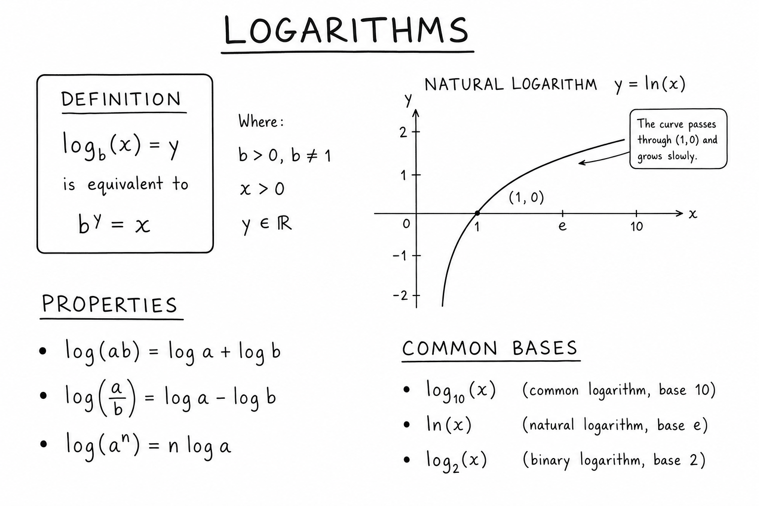
The logarithm with base \(b\) of \(x\) is the exponent you must raise \(b\) to in order to get \(x\):

$$\log_b(x) = y \iff b^y = x$$

So \(\log_2(8) = 3\) because \(2^3 = 8\). \(\log_{10}(1000) = 3\) because \(10^3 = 1000\). \(\log_5(125) = 3\) because \(5^3 = 125\).

The base \(b\) must be positive and not equal to 1. The argument \(x\) must be positive (logs of zero or negative real numbers are undefined in the real number system, though they extend to complex numbers). The output \(y\) can be any real number, positive, negative, or zero.

Three Common Bases

Three logarithm bases dominate practical work:

• \(\log_{10}(x)\): the common logarithm, written simply as \(\log(x)\) in many engineering and science contexts. Used for pH, decibel scales, the Richter magnitude scale, and order-of-magnitude estimates.
• \(\ln(x)\): the natural logarithm, base \(e \approx 2.71828\). Used in calculus, physics, biology, and any context where continuous growth or exponential decay matters.
• \(\log_2(x)\): the binary logarithm. Used in computer science (algorithm complexity, bits of information), information theory, and music theory (octaves are factors of 2).

Different fields default to different bases. Always check the convention before assuming what \(\log\) without a subscript means — it’s base 10 in most engineering, base \(e\) in much of mathematics, and base 2 in computer science.

The Inverse Pair

Exponentiation and logarithm are inverse operations:

$$b^{\log_b(x)} = x \quad \text{and} \quad \log_b(b^x) = x$$

So they undo each other. This is the structural reason logarithms exist — they let you “extract” exponents from expressions where exponents would otherwise be hard to handle.

This inverse relationship is why solving \(2^x = 32\) takes one step (apply \(\log_2\) to both sides) and is why exponential equations in general bend cleanly to logarithmic methods.

Worked Example: Solving an Exponential Equation

Solve \(3 \cdot 2^x = 96\). Divide by 3: \(2^x = 32\). Apply \(\log_2\) to both sides: \(x = \log_2(32) = 5\).

For non-clean numbers, use a calculator and the change of base formula. Solve \(7^x = 50\): \(x = \log_7(50) = \log(50)/\log(7) \approx 1.6990/0.8451 \approx 2.011\).

This is the standard recipe for any exponential equation: isolate the exponential, apply the matching logarithm, simplify. Without logarithms, these problems require trial-and-error or specialized iterative methods. With logarithms, they’re one-line algebra.

The Seven Core Rules

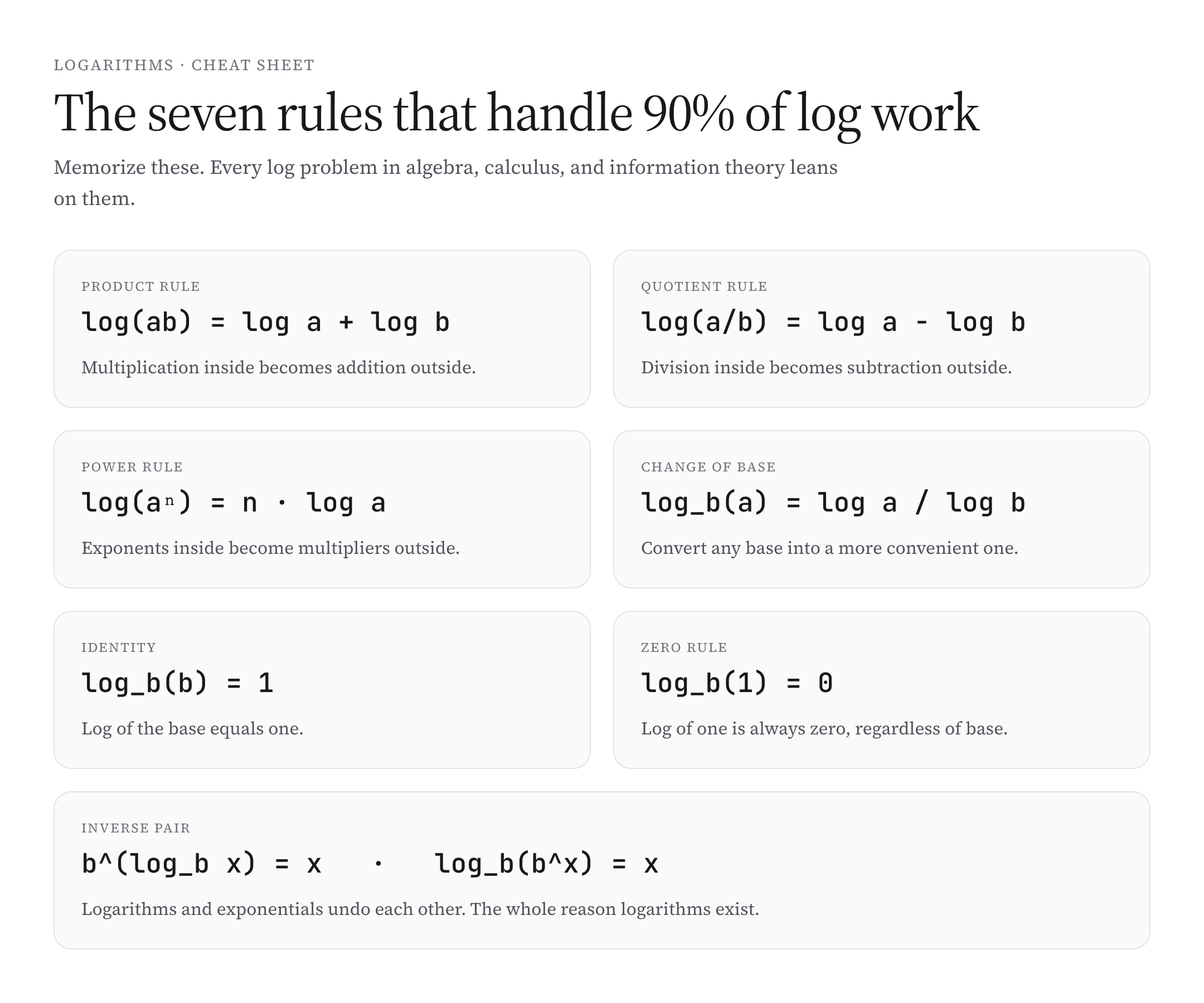
1. Product rule: \(\log_b(xy) = \log_b(x) + \log_b(y)\). Multiplication inside becomes addition outside.
2. Quotient rule: \(\log_b(x/y) = \log_b(x) – \log_b(y)\). Division inside becomes subtraction outside.
3. Power rule: \(\log_b(x^n) = n \log_b(x)\). Exponents inside become multipliers outside.
4. Change of base: \(\log_b(x) = \log_a(x) / \log_a(b)\) for any positive base \(a \neq 1\).
5. Identity: \(\log_b(b) = 1\). The log of the base equals one.
6. Zero rule: \(\log_b(1) = 0\). The log of one is always zero, regardless of base.
7. Inverse pair: \(b^{\log_b(x)} = x\) and \(\log_b(b^x) = x\). The two operations cancel each other.

These seven rules cover virtually every algebraic manipulation you’ll do with logarithms. Memorize them and verify by checking simple numerical examples until they become automatic.

Change of Base in Practice

Most calculators only have buttons for \(\log_{10}\) and \(\ln\). To compute \(\log_b(x)\) for any other base, use:

$$\log_b(x) = \frac{\log(x)}{\log(b)} = \frac{\ln(x)}{\ln(b)}$$

Either common log or natural log works in the change of base formula — pick whichever is more convenient. The result is the same.

For example, \(\log_2(1000) = \log(1000)/\log(2) = 3/0.301 \approx 9.97\). So you’d need just under 10 doublings to grow from 1 to 1000.

Worked Example: Combining Log Rules

Simplify \(\log(8x^2 / y^3)\):

$$\log(8x^2 / y^3) = \log(8) + \log(x^2) – \log(y^3)$$ $$= \log(8) + 2\log(x) – 3\log(y)$$ $$= 3\log(2) + 2\log(x) – 3\log(y)$$

The product, quotient, and power rules combine to break a complicated logarithm into manageable pieces. This kind of simplification is the bread and butter of using logarithms in calculus and applied math, where you want to expose the underlying structure of an expression before differentiating, integrating, or analyzing it.

Linear Scale vs Logarithmic Scale

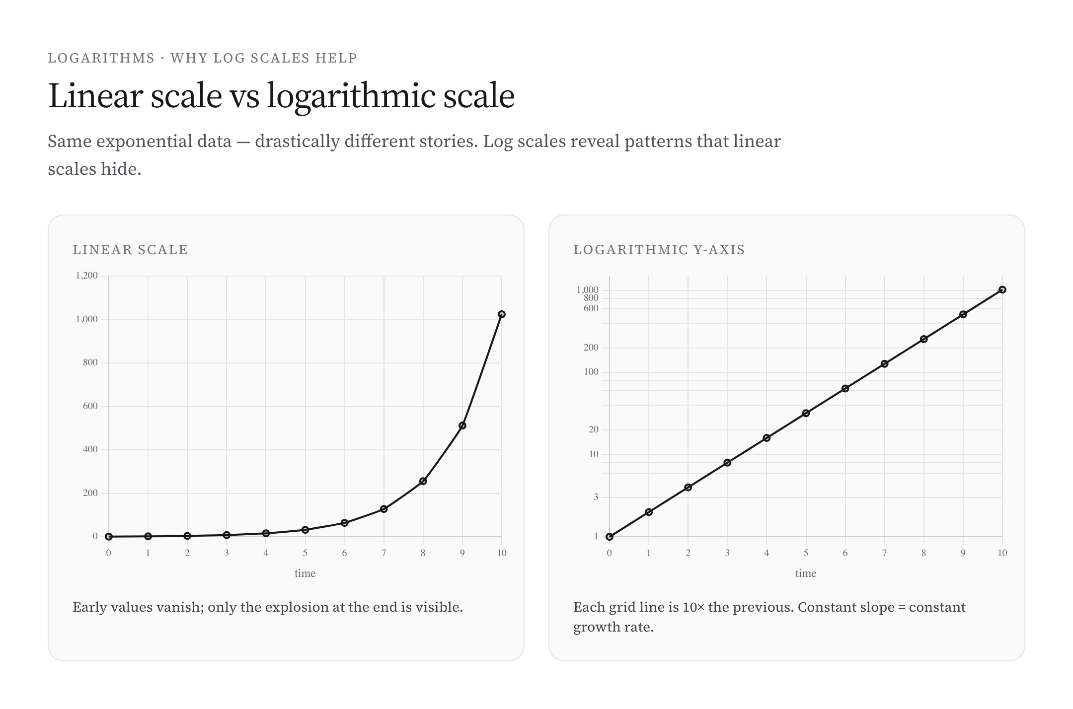
Many real-world quantities span enormous ranges — sound intensity from a whisper to a jet engine, light intensity from starlight to noon sunlight, earthquake magnitudes from imperceptible to devastating. Plotting them on a linear scale either compresses the small values into invisibility or makes the large values run off the chart.

Logarithmic scales solve the problem. Each unit on a log scale represents a multiplicative factor (typically 10×), so a factor of a million spans only six log units. Constant-percentage growth shows up as a straight line on a semi-log plot, which is why financial returns, biological growth, and Moore’s law are usually plotted on log scales.

If you ever see a chart where the y-axis labels go 1, 10, 100, 1000, 10000 with even spacing, you’re looking at a log scale. The interpretation rules are different from linear scales — slopes mean growth rates, not absolute differences.

Applications: Decibels and pH

The decibel scale measures sound intensity logarithmically:

$$L = 10 \log_{10}(I / I_0)$$

Each 10 dB increase corresponds to 10× the sound intensity. A 90 dB jackhammer is a billion times more intense than the 0 dB threshold of hearing — a number that’s intuitive on the dB scale and unmanageable on a linear scale.

The pH scale is similarly logarithmic:

$$\text{pH} = -\log_{10}([H^+])$$

Each pH unit represents a 10× change in hydrogen ion concentration. Lemon juice (pH 2) is 10,000× more acidic than coffee (pH 6). Logarithmic scales are everywhere in chemistry, biology, geology, and astronomy precisely because real natural quantities span huge ranges.

Applications: Computer Science

Algorithm complexity uses logarithms constantly. Binary search is \(O(\log n)\) because each step halves the search space. Heap operations are \(O(\log n)\) for the same reason. Efficient sorting algorithms (merge sort, heapsort) achieve \(O(n \log n)\) — provably optimal for comparison-based sorting.

Information theory uses base-2 logarithms to measure information content in bits. The Shannon entropy of a discrete distribution is \(H = -\sum p_i \log_2(p_i)\). The number of bits needed to encode \(n\) equally likely outcomes is \(\log_2(n)\). Whenever bits and information get measured, logarithms appear.

Applications: Calculus and Continuous Growth

The natural logarithm \(\ln(x)\) emerges naturally in calculus. Its derivative is \(1/x\), and its inverse \(e^x\) is the unique function whose derivative equals itself. Together they govern continuous growth and decay — radioactive half-lives, capacitor discharge, population growth, compound interest, drug clearance from the bloodstream.

Continuous compound interest computes balance as \(B = P e^{rt}\). Solving for time given a target balance uses the natural log: \(t = \ln(B/P) / r\). Half-life calculations use \(t_{1/2} = \ln(2) / k\). Anywhere continuous exponential change happens, the natural log is the inverse that retrieves time or rate from amount.

Logarithms in Finance

Compound interest grows exponentially, so financial analysis uses logarithms heavily. The continuously compounded return over a period is \(\ln(P_{\text{end}} / P_{\text{start}})\). Log returns are additive across periods, which makes them more mathematically convenient than simple percentage returns for portfolio modeling and time-series analysis.

The Black-Scholes option pricing model assumes log-normal distribution of asset prices — meaning the logarithm of the price follows a normal distribution. Many financial risk models use log returns precisely because the additive property simplifies aggregation across time and assets.

Common Mistakes With Logarithms

1. \(\log(a + b) \neq \log(a) + \log(b)\). The rule applies to multiplication, not addition. \(\log(2 + 3) = \log(5) \neq \log(2) + \log(3)\).
2. Confusing \(\log(x^2)\) with \((\log x)^2\). The first equals \(2 \log x\); the second is the log squared. Different operations.
3. Taking logs of negative numbers. \(\log(-5)\) is undefined for real numbers. Logs extend to complex numbers but introduce additional complexity (multi-valuedness).
4. Forgetting which base. “Log” without a subscript is ambiguous — base 10 in engineering, base \(e\) in mathematics, base 2 in computer science. Specify the base when context is unclear.
5. Mishandling \(\log(1)\). Always zero, regardless of base. Easy to forget when working through algebra.
6. Ignoring the domain. The argument of a log must be positive. Equations involving logs may have spurious “solutions” that violate the domain — always check.

A Brief History of Logarithms

John Napier introduced logarithms in 1614 in his work Mirifici Logarithmorum Canonis Descriptio. His goal was practical — to turn multiplication into addition for astronomical calculations. Henry Briggs adopted base 10 a few years later, producing the first comprehensive log tables in 1617 (3-digit) and 1624 (14-digit).

Logarithms revolutionized computation. Slide rules, based on log scales, became the standard engineering tool for over 300 years until pocket calculators displaced them in the 1970s. Pierre-Simon Laplace credited logarithms with “doubling the life of an astronomer.”

The natural logarithm and the constant \(e\) emerged from independent work by Jacob Bernoulli (compound interest, 1683) and the calculus of Newton and Leibniz (1670s–80s). Today logarithms are still essential — every science, engineering, and computer science discipline uses them, even though the actual computation is now hidden inside calculators and software.

Logarithmic Differentiation

For complex products, quotients, and powers, taking the natural log first simplifies differentiation. To differentiate \(y = x^x\), take \(\ln\) of both sides: \(\ln y = x \ln x\). Differentiate implicitly: \(y’/y = \ln x + 1\). So \(y’ = x^x (\ln x + 1)\).

Logarithmic differentiation is the standard tool whenever a function has variables in both base and exponent, or whenever a product or quotient of many factors needs to be differentiated. It converts multiplications into additions and exponentials into multiplications, dramatically simplifying the derivative computation.

Information Theory and Entropy

Shannon’s entropy of a discrete probability distribution is \(H = -\sum p_i \log_2(p_i)\). The base-2 logarithm gives entropy in bits — the average number of binary digits needed to encode an outcome.

Entropy underpins data compression (gzip, JPEG, MP3 all reduce file sizes toward the entropy lower bound), machine learning (cross-entropy loss measures how far model predictions are from true distributions), and channel capacity in communications. Anywhere quantitative information matters, logarithmic measures appear because logs are the natural way to count “amount of choice” or “amount of uncertainty.”

History of Slide Rules and Log Tables

Before electronic calculators, the slide rule was the engineer’s universal computational tool. Two sliding wooden or plastic rules with logarithmic scales let you multiply and divide huge numbers by adding or subtracting lengths. The slide rule dominated science and engineering for over 300 years, from the early 1600s until pocket calculators arrived in the 1970s.

NASA engineers used slide rules to compute trajectories for the Apollo missions. K&E and Pickett were the major manufacturers. The standard “log-log duplex” model handled exponentials, trigonometry, and roots in addition to multiplication and division. Mastering a slide rule was a rite of passage for engineering students until the HP-35 calculator (1972) made the technology obsolete almost overnight.

Log Returns vs Simple Returns in Finance

Simple returns compute price change as a percentage: \((P_t – P_{t-1}) / P_{t-1}\). Log returns use the natural log: \(\ln(P_t / P_{t-1})\). For small changes the two are nearly identical; for large changes they diverge.

Log returns have two big advantages. First, they’re additive across time: a sequence of log returns sums to the total log return over the period. Simple returns multiply geometrically and don’t sum. Second, log returns are usually closer to symmetric (a 50% gain followed by a 50% loss leaves you down 25% in simple terms but exactly back to zero in log terms when paired with the matching log return). For long-horizon time-series modeling, log returns are the standard.

Why Calculators Have Both LOG and LN Buttons

Most scientific calculators have separate LOG (base 10) and LN (base e) buttons. The reason: each base is the natural choice for different problem domains. LOG is used for engineering scales (decibels, pH, Richter, slide-rule arithmetic). LN is used for calculus, physics, biology, and continuous-growth problems where the natural exponential \(e^x\) appears.

Both buttons are technically redundant — the change-of-base formula converts between them. But having both saves a step in routine calculations, and the redundancy reflects the historical reality that these two bases dominate practical work in different fields. Computer scientists sometimes wish for a third LOG2 button, since binary logarithms appear constantly in algorithm complexity, but most calculators omit it.

Common Worked Examples Worth Memorizing

A few standard log calculations come up so often they’re worth memorizing as facts:

• \(\log_{10}(2) \approx 0.301\). Useful for back-of-envelope conversions between binary and decimal.
• \(\log_{10}(3) \approx 0.477\). Combined with log 2, lets you compute logs of any small integer composed of 2s and 3s.
• \(\ln(2) \approx 0.693\). Half-life calculations: \(t_{1/2} = \ln(2) / k\). Doubling time: \(t_{2x} = \ln(2) / r\) for continuous growth rate \(r\).
• \(\log_2(10) \approx 3.32\). The number of bits needed to represent a single decimal digit. \(\log_2(1000) \approx 9.97\), so 10 bits cover 1024 — close to 1000.
• The “Rule of 70” (or sometimes 72): doubling time at growth rate \(r\) is approximately \(70/r\) periods. Derived from \(\ln(2) \approx 0.693\) ≈ 0.70.

These shortcuts speed up financial estimates, biology calculations, and back-of-envelope reasoning enormously.

FAQs