Limits in Calculus

Limits in calculus describe what a function approaches as the input approaches a particular value. They’re the bridge between algebra and calculus. Without limits, derivatives wouldn’t exist, integrals wouldn’t be defined, and continuity would be a vibes-based notion. Once limits click, the rest of calculus stops feeling like magic and starts feeling like bookkeeping.

Most students stumble on the formal definition first. The trick is to grasp the intuition before wrestling with epsilons and deltas. After that, the limit laws turn most calculations into routine algebra, and the few weird cases (indeterminate forms, infinite limits, asymptotic behavior) get their own clean techniques.

This study note walks through the intuitive definition, the formal epsilon-delta version, the limit laws you’ll actually use, one-sided limits, infinite limits, indeterminate forms and L’Hopital’s rule, continuity, and the historical and modern context that explains why limits became the foundation of analysis.

The Intuitive Definition of Limits in Calculus

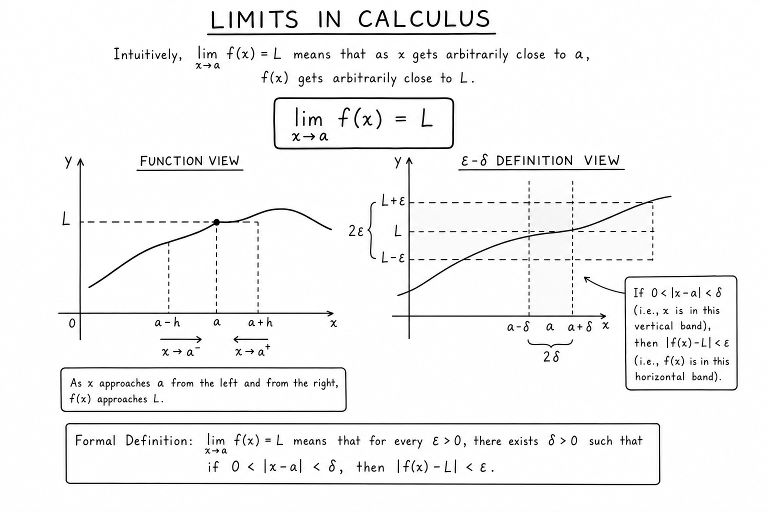
The limit of \(f(x)\) as \(x\) approaches \(a\) is the value \(L\) that the function gets arbitrarily close to as \(x\) gets close to \(a\) from either side:

$$\lim_{x \to a} f(x) = L$$

Notice what’s missing: the function doesn’t have to actually equal \(L\) at \(x = a\). It doesn’t even have to be defined at \(a\). The limit only cares about behavior near the point, not at the point.

That distinction is the whole reason limits exist. They let you ask “where is this function heading?” without requiring it to arrive. The classic example: \(f(x) = (x^2 – 1)/(x – 1)\) is undefined at \(x = 1\) (you’d be dividing by zero), but \(\lim_{x \to 1} f(x) = 2\) because the function simplifies to \(x + 1\) for every \(x \neq 1\), and that simplified function clearly approaches 2.

The Epsilon-Delta Definition

The formal version: \(\lim_{x \to a} f(x) = L\) means that for every \(\varepsilon > 0\), there exists a \(\delta > 0\) such that:

$$0 < |x - a| < \delta \implies |f(x) - L| < \varepsilon$$

In English: pick any tolerance \(\varepsilon\) for how close \(f(x)\) should be to \(L\). I can give you a window \(\delta\) around \(a\) where the function stays inside that tolerance. If I can do that for every \(\varepsilon\), the limit equals \(L\).

This is the rigorous foundation. You’ll rarely use it directly after first-year calc, but every limit law and every theorem about continuity reduces back to this definition. Augustin-Louis Cauchy popularized this approach in the 1820s, and Karl Weierstrass made it fully rigorous in the 1870s, ending nearly two centuries of fuzzy reasoning about infinitesimals.

Limit Laws

For limits that exist, the standard rules let you break complex expressions into pieces:

• Sum: \(\lim (f + g) = \lim f + \lim g\)
• Product: \(\lim (f \cdot g) = \lim f \cdot \lim g\)
• Quotient: \(\lim (f/g) = \lim f / \lim g\), provided \(\lim g \neq 0\)
• Constant multiple: \(\lim (c \cdot f) = c \cdot \lim f\)
• Power: \(\lim f^n = (\lim f)^n\)
• Composition: \(\lim_{x \to a} f(g(x)) = f(\lim_{x \to a} g(x))\) when \(f\) is continuous at the inner limit

For continuous functions, you can substitute directly: \(\lim_{x \to a} f(x) = f(a)\). That’s the entire point of continuity. Polynomials, exponentials, sines, and cosines are all continuous everywhere, so direct substitution works whenever the result isn’t an indeterminate form.

One-Sided Limits

Approaching from the left: \(\lim_{x \to a^-} f(x)\). From the right: \(\lim_{x \to a^+} f(x)\). The two-sided limit exists only when both one-sided limits exist and agree.

This is how piecewise functions break: if the left and right limits at a junction don’t match, the function has a jump discontinuity and no limit at that point. Step functions, the floor function, and the absolute value function all live and die by one-sided limit behavior.

One-sided limits also matter at the boundaries of a function’s domain. The square root function \(\sqrt{x}\) only has a right-sided limit at \(x = 0\) because the function isn’t defined for negative \(x\). Most calculus textbooks count this as the limit existing, even though no two-sided limit can technically be defined.

Infinite Limits and Limits at Infinity

Two related but distinct ideas. Infinite limits describe functions that grow without bound near a point: \(\lim_{x \to 0} 1/x^2 = \infty\). The notation conveys that the function diverges; strictly speaking, the limit doesn’t exist as a real number.

Limits at infinity describe long-run behavior: \(\lim_{x \to \infty} f(x) = L\) means \(f(x)\) approaches \(L\) as \(x\) grows without bound. These show up in horizontal asymptote analysis. Rational functions like \(f(x) = (3x^2 + 2)/(x^2 + 5)\) have horizontal asymptotes given by the ratio of leading coefficients: \(\lim_{x \to \infty} f(x) = 3\).

Both ideas are routinely combined: \(\lim_{x \to \infty} e^x = \infty\), \(\lim_{x \to -\infty} e^x = 0\). Together they describe the full asymptotic behavior of most functions you’ll meet.

Indeterminate Forms and L’Hopital’s Rule

Some limits look like they should be undefined but aren’t:

• \(0/0\) — needs algebraic simplification or L’Hopital’s rule
• \(\infty / \infty\) — same treatment
• \(0 \cdot \infty\), \(\infty – \infty\), \(0^0\), \(\infty^0\), \(1^\infty\) — rewrite first to expose a 0/0 or ∞/∞ form, then apply L’Hopital

L’Hopital’s rule: if \(\lim f(x)\) and \(\lim g(x)\) both equal 0 or both equal ∞, then:

$$\lim \frac{f(x)}{g(x)} = \lim \frac{f'(x)}{g'(x)}$$

provided the right-hand limit exists. Apply repeatedly if needed. The classic example: \(\lim_{x \to 0} \frac{\sin x}{x} = \lim_{x \to 0} \frac{\cos x}{1} = 1\). The squeeze theorem and Taylor series both prove the same result without L’Hopital, and one of them is usually faster in practice.

Continuity and the Intermediate Value Theorem

A function is continuous at \(a\) when \(\lim_{x \to a} f(x) = f(a)\). All three pieces matter: the limit must exist, the function must be defined at \(a\), and they must agree.

Continuous functions inherit nice properties. The Intermediate Value Theorem says that if \(f\) is continuous on \([a, b]\) and \(N\) is between \(f(a)\) and \(f(b)\), then there exists at least one \(c \in (a, b)\) with \(f(c) = N\). This is how root-finding works: locate a sign change in a continuous function, and a root is guaranteed in between.

The Extreme Value Theorem guarantees that a continuous function on a closed interval attains its maximum and minimum somewhere on that interval. These two theorems are the foundation for most existence proofs in single-variable calculus.

The Squeeze Theorem

If \(g(x) \leq f(x) \leq h(x)\) near \(a\), and \(\lim_{x \to a} g(x) = \lim_{x \to a} h(x) = L\), then \(\lim_{x \to a} f(x) = L\).

The squeeze theorem (also called the sandwich theorem) is the cleanest way to evaluate limits where direct methods fail. The textbook example: \(\lim_{x \to 0} x^2 \sin(1/x) = 0\). The function \(\sin(1/x)\) oscillates wildly near zero, so direct evaluation is hopeless. But \(-x^2 \leq x^2 \sin(1/x) \leq x^2\), and both bounds approach 0. The squeeze theorem closes the case.

The squeeze theorem is also the standard tool for proving \(\lim_{x \to 0} \sin(x)/x = 1\) without circular reasoning, which is then used to derive the derivatives of all the trig functions.

Worked Example: A Tricky Limit

Compute \(\lim_{x \to 4} \frac{\sqrt{x} – 2}{x – 4}\).

Direct substitution gives 0/0 — indeterminate. Multiply top and bottom by the conjugate \(\sqrt{x} + 2\):

$$\frac{\sqrt{x} – 2}{x – 4} \cdot \frac{\sqrt{x} + 2}{\sqrt{x} + 2} = \frac{x – 4}{(x – 4)(\sqrt{x} + 2)} = \frac{1}{\sqrt{x} + 2}$$

Now substitute: \(\lim_{x \to 4} \frac{1}{\sqrt{x} + 2} = \frac{1}{4}\). The original expression has the same limit because the simplified form agrees with the original except at \(x = 4\), and limits don’t care what happens at the point.

This conjugate trick handles many limits involving square roots. The general lesson: when you see 0/0, look for an algebraic manipulation (factor, conjugate, common denominator) that exposes the cancellation.

Why Limits Underpin Everything in Calculus

Derivatives are limits of difference quotients:

$$f'(x) = \lim_{h \to 0} \frac{f(x+h) – f(x)}{h}$$

Definite integrals are limits of Riemann sums:

$$\int_a^b f(x)\, dx = \lim_{n \to \infty} \sum_{i=1}^n f(x_i^*) \Delta x$$

Continuity is defined in terms of limits. Convergence of infinite series is defined as the limit of partial sums. Differential equations rely on limit-based definitions of derivatives. Even probability distributions in advanced statistics use limits to define cumulative distribution functions and characteristic functions.

Limits power every other concept in calculus and a huge fraction of higher analysis. Read more in interesting math articles and must-read research papers and Aryabhata’s contributions to mathematics.

Common Mistakes When Computing Limits

1. Plugging in too early. Always check for indeterminate forms first. Direct substitution works for continuous functions, not for everything.
2. Forgetting one-sided behavior. A function might have left and right limits that disagree. The two-sided limit exists only when they match.
3. Misapplying L’Hopital. The rule requires both numerator and denominator to give 0/0 or ∞/∞. Applying it to other forms produces wrong answers.
4. Cancelling factors at the limit point. When \(x \to a\), you can cancel factors that equal zero at \(a\) — but only because the limit doesn’t care about the value at \(a\). Be explicit about that step.
5. Confusing infinite limits with limits that don’t exist. “The limit is infinity” is a way of saying the function diverges; the formal limit doesn’t exist as a real number.
6. Ignoring the domain. A function with a restricted domain may have only one-sided limits at the boundary. \(\sqrt{x}\) has no two-sided limit at \(x = 0\) because it isn’t defined for negative values.

A Brief History of Limits

The intuition behind limits is ancient. Eudoxus of Cnidus and Archimedes used the “method of exhaustion” in the 4th and 3rd centuries BCE to compute areas and volumes by squeezing them between known approximations — essentially a limit argument without modern notation.

Newton and Leibniz built calculus in the 1670s and 1680s using infinitesimals — quantities smaller than any positive real but greater than zero. The math worked, but the foundations were philosophically suspect. Bishop Berkeley famously called infinitesimals “the ghosts of departed quantities” in 1734.

Cauchy’s Cours d’Analyse (1821) introduced the limit-based foundations that survive today. Karl Weierstrass formalized epsilon-delta arguments in the 1860s and 1870s, and the modern \(\varepsilon-\delta\) definition became the rigorous standard. Abraham Robinson’s nonstandard analysis (1960) rehabilitated infinitesimals on rigorous grounds, but the limit approach won the textbook war for pedagogical and computational reasons.

Limits in Multivariable Calculus and Beyond

In multivariable calculus, limits become subtler because there are infinitely many paths to approach a point. \(\lim_{(x,y) \to (0,0)} f(x, y) = L\) requires \(f\) to approach \(L\) along every possible path. If two paths give different limits, the multivariable limit doesn’t exist.

This is why \(f(x, y) = xy / (x^2 + y^2)\) has no limit at the origin: along \(y = 0\), the function is 0; along \(y = x\), the function is 1/2. Different paths give different values, so the multivariable limit fails.

In topology and analysis, limits generalize even further to convergence of sequences in metric spaces, nets in topological spaces, and filters in category theory. The basic insight — what value is the system approaching as a parameter varies? — keeps showing up across every branch of mathematics.

Continuous Functions and the Composition Rule

The composition of continuous functions is continuous: if \(g\) is continuous at \(a\) and \(f\) is continuous at \(g(a)\), then \(f \circ g\) is continuous at \(a\). This is why \(\sin(x^2)\), \(e^{\cos x}\), and \(\ln(1 + x^2)\) are continuous everywhere they’re defined — they’re built from continuous primitives composed together.

The composition rule is also why direct substitution works for so many limits. If both the inner function and the outer function are continuous at the limit point, you can just plug in. Trouble arises only when one of them is discontinuous, and that’s when you reach for L’Hopital, algebraic manipulation, or the squeeze theorem.

Limits of Sequences vs Functions

The limit of a sequence \(a_n\) as \(n \to \infty\) is conceptually similar to the limit of a function as \(x \to \infty\), but with discrete steps. Definition: \(\lim_{n \to \infty} a_n = L\) if for every \(\varepsilon > 0\) there exists \(N\) such that \(|a_n – L| < \varepsilon\) for all \(n > N\).

Sequence limits underpin convergence of infinite series and the formal definition of integrals as Riemann sum limits. Convergence tests for series — comparison test, ratio test, root test, integral test — all rely on understanding sequence limit behavior.

How to Avoid Circular Reasoning When Proving Limits

Common circular trap: using L’Hopital’s rule to prove \(\lim_{x \to 0} \sin(x)/x = 1\). L’Hopital’s rule requires knowing the derivative of \(\sin x\). The derivative of \(\sin x\) is proven using the limit \(\sin(x)/x \to 1\). Circular.

The standard non-circular proof uses the squeeze theorem and elementary geometry: comparing the area of a triangle, sector, and bigger triangle inscribed in the unit circle gives \(\sin x \le x \le \tan x\) for small positive \(x\). Dividing by \(\sin x\) and taking the limit yields the result. Many calculus textbook proofs are subtly circular until checked carefully against the order of derivation.

Convergence Speed and Asymptotic Analysis

Two functions can both have the same limit but approach it at very different speeds. \(\lim_{x \to \infty} 1/x = 0\) and \(\lim_{x \to \infty} e^{-x} = 0\), but \(e^{-x}\) approaches zero exponentially fast while \(1/x\) approaches it only like a power of \(x\).

Asymptotic analysis quantifies these rates with big-O, big-Omega, and big-Theta notation. \(f(x) = O(g(x))\) means \(f\) grows no faster than \(g\) up to a constant factor. This language is the bridge from limits in calculus to algorithm complexity analysis in computer science. Limits give the destination; asymptotic notation describes the path.

FAQs