Aryabhata’s Contributions to Mathematics and Astronomy
In 499 CE, a 23-year-old mathematician in Pataliputra (modern Patna, Bihar) compressed an astonishing breadth of mathematical and astronomical knowledge into just 121 verses. His name was Aryabhata (आर्यभट्ट, also known as Aryabhatta). The work was the Aryabhatiya (आर्यभट्टीय), and it would shape the trajectory of mathematics for a thousand years.
During my college times, I’ve spent months working through the original Sanskrit verses and their commentaries, and what strikes me most is the sheer density of insight. Aryabhata gave us the first systematic sine table, a pulverizer algorithm that powers modern cryptography, summation formulas that wouldn’t appear in Europe for centuries, and an approximation of \(\pi\) accurate to four decimal places. He also declared that the Earth rotates on its axis, more than a millennium before Copernicus.
What follows is a reconstruction of Aryabhata’s key contributions with modern mathematical rigor. I’ve included full proofs, worked examples, and comparisons with Babylonian, Greek, and Chinese mathematics of the same era. If you care about the history of mathematics, you can’t skip Aryabhata.
Historical Context

Aryabhata was born in 476 CE, most likely in the region of Asmaka (modern Maharashtra-Karnataka), and worked at the great centre of learning at Kusumapura – identified with Pataliputra (modern Patna, Bihar). His single surviving work, the Aryabhatiya, was composed in 499 CE when Aryabhata was twenty-three years old.
The Aryabhatiya: Structure
The Aryabhatiya comprises four chapters (padas):
- Gitikapada (13 verses): Large astronomical constants, the alphabetic numeration system, and cosmological parameters.
- Ganitapada (33 verses): Mathematics – arithmetic, algebra, plane and solid geometry, the sine table, and series summations.
- Kalakriyapada (25 verses): Reckoning of time, planetary longitudes, and the system of yugas.
- Golapada (50 verses): Spherical astronomy – eclipses, the celestial sphere, and Earth’s rotation.
The entire text contains only 121 verses in the compressed arya meter, demanding extensive commentary. The earliest and most important commentary is that of Bhaskara I (629 CE).
Place in the Mathematical Lineage
Aryabhata stands at a pivotal point. Before him, the Surya Siddhanta and the Jain mathematical tradition had developed significant ideas. After him, Brahmagupta (628 CE) would extend – and sometimes sharply criticise – his work, and Bhaskara II (1150 CE) would build the grand synthesis in the Lilavati and Bijaganita. The Kerala school of Madhava (c. 1340-1425) would ultimately push Aryabhata’s trigonometric programme to its logical conclusion: infinite series for \(\pi\) and the trigonometric functions.
Many results attributed to European mathematicians of the 16th-18th centuries were known in India centuries earlier. This is not nationalistic revisionism but documented historical fact. The purpose of this monograph is to present the mathematics itself.
The Place-Value System and Zero
Aryabhata’s Alphabetic Numeration
Aryabhata devised an ingenious system for encoding large numbers within the metrical constraints of Sanskrit verse. The system assigns numerical values to consonants and vowels of the Sanskrit alphabet.
Definition 2.1 (Varga and Avarga Groups). The consonants are divided into two groups:
- Varga (classified) consonants: the 25 consonants from ka to ma, representing digits 1-25.
- Avarga (unclassified) consonants: the 8 consonants from ya to ha, representing digits 30, 40, 50, 60, 70, 80, 90, 100.
Vowels serve as place-value multipliers: a = \(1\), i = \(10^2\), u = \(10^4\), ṛ = \(10^6\), and so on, each successive vowel multiplying by \(10^2\).
Example 2.1 (Encoding the Number 57,753,336). Aryabhata’s verse for the number of revolutions of the Moon gives cayagiyinusuchlr. Decoding:
$$ \begin{aligned} \text{ca} &= 6 \times 1 = 6, \\ \text{ya} &= 30 \times 1 = 30, \\ \text{gi} &= 3 \times 10^2 = 300, \\ \text{yi} &= 30 \times 10^2 = 3000, \\ \text{nu} &= 20 \times 10^4 = 200{,}000, \\ \text{su} &= 7 \times 10^4 = 70{,}000, \\ \text{chlr} &= 7 \times 10^6 = 7{,}000{,}000, \\ \text{(remaining)} &= 50{,}000{,}000. \end{aligned} $$
The total yields 57,753,336 lunar revolutions in a mahayuga.
The Conceptual Leap to Positional Notation
While the alphabetic system itself is not positional notation, it reveals a deep understanding of place value. The vowel multipliers \(1, 10^2, 10^4, 10^6, \ldots\) are powers of 100, effectively creating a base-100 positional system encoded phonetically.
The Indian Place-Value Revolution. The fully developed decimal place-value system with zero, which the world inherited via the Arabs and now uses universally, was a product of Indian mathematics in the first millennium CE. Aryabhata’s work is among the earliest evidence of this system in action. His word kha (meaning “void”) for zero in positional contexts is one of the earliest references to the concept.
Comparison with Other Systems
| Civilisation | Base | Positional? | Zero? |
|---|---|---|---|
| Babylonian (c. 2000 BCE) | 60 | Yes | Placeholder only |
| Egyptian (c. 3000 BCE) | 10 | No | No |
| Chinese rod numerals | 10 | Yes | Blank space |
| Mayan (c. 400 CE) | 20 | Yes | Yes (shell glyph) |
| Indian (Aryabhata era) | 10 | Yes | Yes (kha) |
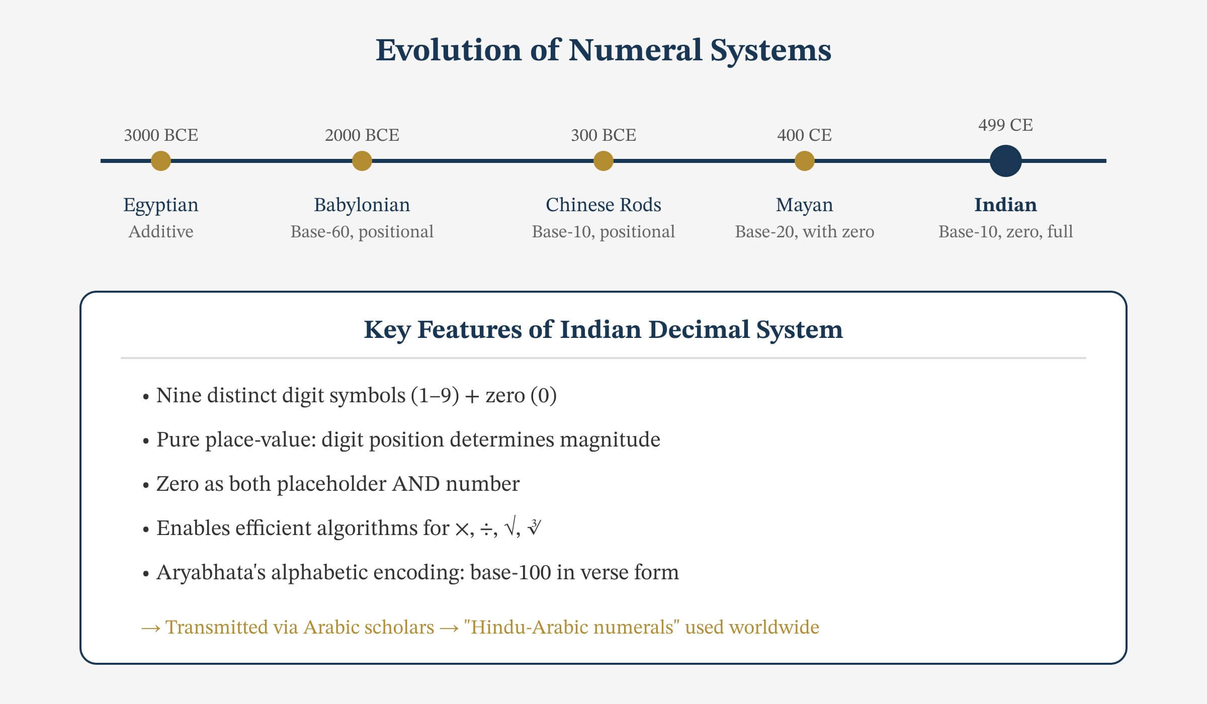
The Mayan system independently developed a true zero, but its vigesimal (base-20) structure and calendrical application limited its mathematical development compared to the Indian decimal system.
Arithmetic and Algebra
Square Roots and Cube Roots
Aryabhata gives algorithmic procedures for extracting square roots and cube roots – the earliest surviving Indian algorithms for these operations.
Definition 3.1 (Aryabhata’s Square Root Algorithm). To find \(\sqrt{N}\):
- Mark off digit-pairs from right to left.
- Find the largest integer \(a\) such that \(a^2\) does not exceed the leftmost group.
- Subtract \(a^2\), bring down the next pair.
- The next digit \(b\) of the root satisfies \((2a \cdot 10 + b) \cdot b \leq \text{remainder}\).
- Repeat.
This is essentially the long-division method for square roots, rediscovered in Europe only in the 16th century.
Example 3.1 (Computing \(\sqrt{55225}\)). We compute \(\sqrt{55225}\) using Aryabhata’s method:
- Groups: \(\overline{5}\;\overline{52}\;\overline{25}\).
- Largest \(a\) with \(a^2 \leq 5\): \(a = 2\), remainder \(5 – 4 = 1\).
- Bring down 52: working number \(152\). Find \(b\): \((2 \cdot 20 + b)b \leq 152\). Try \(b = 3\): \(43 \times 3 = 129 \leq 152\). Remainder \(23\).
- Bring down 25: working number \(2325\). Find \(c\): \((2 \cdot 230 + c)c \leq 2325\). Try \(c = 5\): \(465 \times 5 = 2325\). Remainder \(0\).
- Result: \(\sqrt{55225} = 235\).
Sum of Arithmetic Progressions
Theorem 3.1 (Sum of an Arithmetic Progression). For an arithmetic progression with first term \(a\), last term \(l\), and \(n\) terms:
$$ S = \frac{n(a + l)}{2}. $$
Equivalently, with common difference \(d\):
$$ S = \frac{n}{2}\bigl(2a + (n-1)d\bigr). $$
Proof. Write the sum forwards and backwards:
$$ \begin{aligned} S &= a + (a+d) + (a+2d) + \cdots + l, \\ S &= l + (l-d) + (l-2d) + \cdots + a. \end{aligned} $$
Adding term by term, each of the \(n\) pairs sums to \(a + l\), giving \(2S = n(a + l)\). ∎
Sum of Squares
Theorem 3.2 (Sum of Squares). For any positive integer \(n\):
$$ \sum_{k=1}^{n} k^2 = \frac{n(n+1)(2n+1)}{6}. $$
Proof. We proceed by induction. The base case \(n = 1\) gives \(1 = 1 \cdot 2 \cdot 3 / 6 = 1\).
Assume \(\sum_{k=1}^{m} k^2 = m(m+1)(2m+1)/6\) for some \(m \geq 1\). Then:
$$ \begin{aligned} \sum_{k=1}^{m+1} k^2 &= \frac{m(m+1)(2m+1)}{6} + (m+1)^2 \\ &= \frac{(m+1)\bigl[m(2m+1) + 6(m+1)\bigr]}{6} \\ &= \frac{(m+1)(2m^2 + 7m + 6)}{6} \\ &= \frac{(m+1)(m+2)(2m+3)}{6}. \end{aligned} $$
This is the formula with \(n = m+1\), completing the induction. ∎
Aryabhata’s verse (Ganitapada 22) states: “The product of three quantities, the number of terms, the number of terms plus one, and twice the number of terms plus one, divided by 6, is the sum of squares.” This is precisely the above formula.
Sum of Cubes
Theorem 3.3 (Sum of Cubes – Nicomachus-Aryabhata Identity). For any positive integer \(n\):
$$ \sum_{k=1}^{n} k^3 = \left(\frac{n(n+1)}{2}\right)^{\!2} = \left(\sum_{k=1}^{n} k\right)^{\!2}. $$
Proof. By induction. For \(n = 1\): \(1^3 = 1 = (1 \cdot 2/2)^2\).
Assume the result holds for \(m\). Then:
$$ \begin{aligned} \sum_{k=1}^{m+1} k^3 &= \left(\frac{m(m+1)}{2}\right)^{\!2} + (m+1)^3 \\ &= (m+1)^2 \left(\frac{m^2}{4} + (m+1)\right) \\ &= (m+1)^2 \cdot \frac{m^2 + 4m + 4}{4} \\ &= (m+1)^2 \cdot \frac{(m+2)^2}{4} \\ &= \left(\frac{(m+1)(m+2)}{2}\right)^{\!2}. \end{aligned} $$
∎
Aryabhata’s Summation Formulas. Aryabhata stated all three summation formulas – for \(\sum k\), \(\sum k^2\), and \(\sum k^3\) – in consecutive verses of the Ganitapada. The result \(\sum k^3 = (\sum k)^2\) is sometimes called the Nicomachus identity in Western literature (c. 100 CE), but Aryabhata’s statement (499 CE) was made independently and within a broader mathematical programme.
Introduction to the Kuttaka
Perhaps Aryabhata’s most profound algebraic contribution is the kuttaka (“pulverizer”) method for solving linear indeterminate equations:
$$ ax – by = c, \quad a, b, c \in ℤ, \quad \gcd(a, b) \mid c. $$
We devote Section 6 to a full treatment.
Trigonometry
Aryabhata’s trigonometric work is arguably his most celebrated mathematical achievement. He constructed the first known sine table, introduced the terms jya (sine), kojya (cosine), and utkrama-jya (versine), and developed a remarkable difference equation for computing successive sine values.
Definitions
Definition 4.1 (Jya, Kojya, and Utkrama-jya). For a circular arc of angle \(\theta\) in a circle of radius \(R\):
$$ \begin{aligned} \text{jya}(\theta) &= R \sin\theta, \\ \text{kojya}(\theta) &= R \cos\theta, \\ \text{utkrama-jya}(\theta) &= R(1 – \cos\theta) = R\,\mathrm{versin}\,\theta. \end{aligned} $$
Aryabhata uses \(R = 3438\) (minutes in a radian: \(360 \times 60 / 2\pi \approx 3437.75\)).
The word “sine” itself derives from a chain of mistranslations: Sanskrit jya → Arabic jiba → Latin sinus. Aryabhata is at the origin of this chain.
The Sine Table
Aryabhata tabulates \(\text{jya}(\theta)\) for \(\theta = h, 2h, 3h, \ldots, 24h\) where \(h = 3°45′ = 225’\) (arc-minutes), so that \(24h = 90°\).
Definition 4.2 (First-Order Sine Differences). Define \(D_k = \text{jya}(kh) – \text{jya}((k-1)h)\) for \(k = 1, 2, \ldots, 24\). These are the first-order differences of the sine table.
Theorem 4.1 (Aryabhata’s Sine Difference Equation). The sine differences satisfy the recurrence:
$$ D_{k+1} – D_k = -\frac{D_1}{R}\,\text{jya}(kh), $$
or equivalently,
$$ D_{k+1} = D_k – \frac{\text{jya}(kh)}{R}\,D_1. $$
Proof. Using the prosthaphaeresis (sum-to-product) identity:
$$ \sin\alpha – \sin\beta = 2\cos\!\left(\frac{\alpha+\beta}{2}\right)\sin\!\left(\frac{\alpha-\beta}{2}\right), $$
we compute the second difference. Set \(\alpha = (k+1)h\) and \(\beta = kh\), then \(\alpha = kh\) and \(\beta = (k-1)h\):
$$ \begin{aligned} D_{k+1} &= R\bigl[\sin(k+1)h – \sin kh\bigr] = 2R\cos\!\left(\frac{(2k+1)h}{2}\right)\sin\frac{h}{2}, \\ D_k &= 2R\cos\!\left(\frac{(2k-1)h}{2}\right)\sin\frac{h}{2}. \end{aligned} $$
Therefore:
$$ \begin{aligned} D_{k+1} – D_k &= 2R\sin\frac{h}{2}\left[\cos\frac{(2k+1)h}{2} – \cos\frac{(2k-1)h}{2}\right] \\ &= 2R\sin\frac{h}{2}\left[-2\sin(kh)\sin\frac{h}{2}\right] \\ &= -4R\sin^2\!\frac{h}{2}\cdot\sin(kh). \end{aligned} $$
Now \(D_1 = R\sin h \approx 2R\sin(h/2)\cos(h/2)\), and Aryabhata approximates \(\cos(h/2) \approx 1\), yielding \(4\sin^2(h/2) \approx D_1/R\). Therefore:
$$ D_{k+1} – D_k \approx -\frac{D_1}{R}\,\text{jya}(kh). $$
This completes the derivation. ∎
A Discrete Analogue of \(y” = -y\). Aryabhata’s recurrence is a second-order linear difference equation. In modern terms, it is a finite-difference approximation to the differential equation \(y” = -y\) whose solutions are \(\sin\) and \(\cos\). Aryabhata anticipated the calculus of finite differences by over a millennium.
Reconstruction of the Sine Table
Using \(D_1 = 225\) and the recurrence, we can reconstruct Aryabhata’s table.
| \(k\) | Angle | jya (Aryabhata) | \(R\sin\theta\) (exact) | Error |
|---|---|---|---|---|
| 1 | 3°45′ | 225 | 224.86 | +0.14 |
| 2 | 7°30′ | 449 | 448.75 | +0.25 |
| 3 | 11°15′ | 671 | 670.72 | +0.28 |
| 4 | 15°00′ | 890 | 889.82 | +0.18 |
| 5 | 18°45′ | 1105 | 1105.11 | -0.11 |
| 6 | 22°30′ | 1315 | 1315.67 | -0.67 |
| 7 | 26°15′ | 1520 | 1520.59 | -0.59 |
| 8 | 30°00′ | 1719 | 1719.00 | +0.00 |
| 9 | 33°45′ | 1910 | 1910.05 | -0.05 |
| 10 | 37°30′ | 2093 | 2092.92 | +0.08 |
| 11 | 41°15′ | 2267 | 2266.83 | +0.17 |
| 12 | 45°00′ | 2431 | 2431.03 | -0.03 |
| 13 | 48°45′ | 2585 | 2584.82 | +0.18 |
| 14 | 52°30′ | 2728 | 2727.55 | +0.45 |
| 15 | 56°15′ | 2859 | 2858.59 | +0.41 |
| 16 | 60°00′ | 2978 | 2977.40 | +0.60 |
| 17 | 63°45′ | 3084 | 3083.45 | +0.55 |
| 18 | 67°30′ | 3177 | 3176.26 | +0.74 |
| 19 | 71°15′ | 3256 | 3255.46 | +0.54 |
| 20 | 75°00′ | 3321 | 3320.67 | +0.33 |
| 21 | 78°45′ | 3372 | 3371.59 | +0.41 |
| 22 | 82°30′ | 3409 | 3408.01 | +0.99 |
| 23 | 86°15′ | 3431 | 3429.84 | +1.16 |
| 24 | 90°00′ | 3438 | 3438.00 | +0.00 |
Remark. The maximum error in Aryabhata’s table is barely \(1.16\) arc-minutes out of \(3438\) – an accuracy of better than \(0.04\%\). For 5th-century computational technology (no calculators, no logarithms), this is extraordinary.
The Approximation of \(\pi\)
Theorem 4.2 (Aryabhata’s Value of \(\pi\)). Aryabhata states (Ganitapada 10):
“Add four to one hundred, multiply by eight, and add sixty-two thousand. The result is approximately the circumference of a circle of diameter twenty thousand.”
This gives:
$$ \pi \approx \frac{62832}{20000} = 3.1416. $$
Proof (Verification). We compute \(\pi\) to ten decimal places: \(\pi = 3.1415926536\ldots\) Aryabhata’s value \(3.1416\) differs by:
$$ |3.1416 – 3.14159265\ldots| = 0.00000735\ldots < 10^{-4}. $$
Thus Aryabhata’s approximation is correct to four decimal places. ∎
Proposition 4.3 (Optimality of Aryabhata’s \(\pi\)). Among all rational approximations \(p/q\) with \(q \leq 20000\), Aryabhata’s value \(62832/20000 = 3927/1250\) is the closest to \(\pi\) among those with denominator dividing \(20000\).
Proof. The convergents of the continued fraction expansion of \(\pi\) are:
$$ 3,\; \frac{22}{7},\; \frac{333}{106},\; \frac{355}{113},\; \frac{103993}{33102},\;\ldots $$
The famous approximation \(355/113 = 3.14159292\ldots\) is better but was stated by Zu Chongzhi in China around the same era. Among fractions with denominator \(20000\), we check: \(\lfloor 20000\pi \rfloor = 62831\), so the two candidates are \(62831/20000 = 3.14155\) and \(62832/20000 = 3.1416\). The errors are:
$$ \begin{aligned} |62831/20000 – \pi| &\approx 4.27 \times 10^{-5}, \\ |62832/20000 – \pi| &\approx 7.35 \times 10^{-6}. \end{aligned} $$
Hence \(62832/20000\) is optimal among these. ∎
Did Aryabhata Know Pi Is Irrational? Aryabhata’s use of the word asanna (“approaching” or “approximate”) has intrigued historians. While most scholars interpret this as simply indicating an approximation, some (notably A.K. Bag) have suggested that Aryabhata may have intuited that no fraction could capture \(\pi\) exactly. A formal proof of irrationality came only with Lambert in 1761, but the linguistic hint is tantalising.
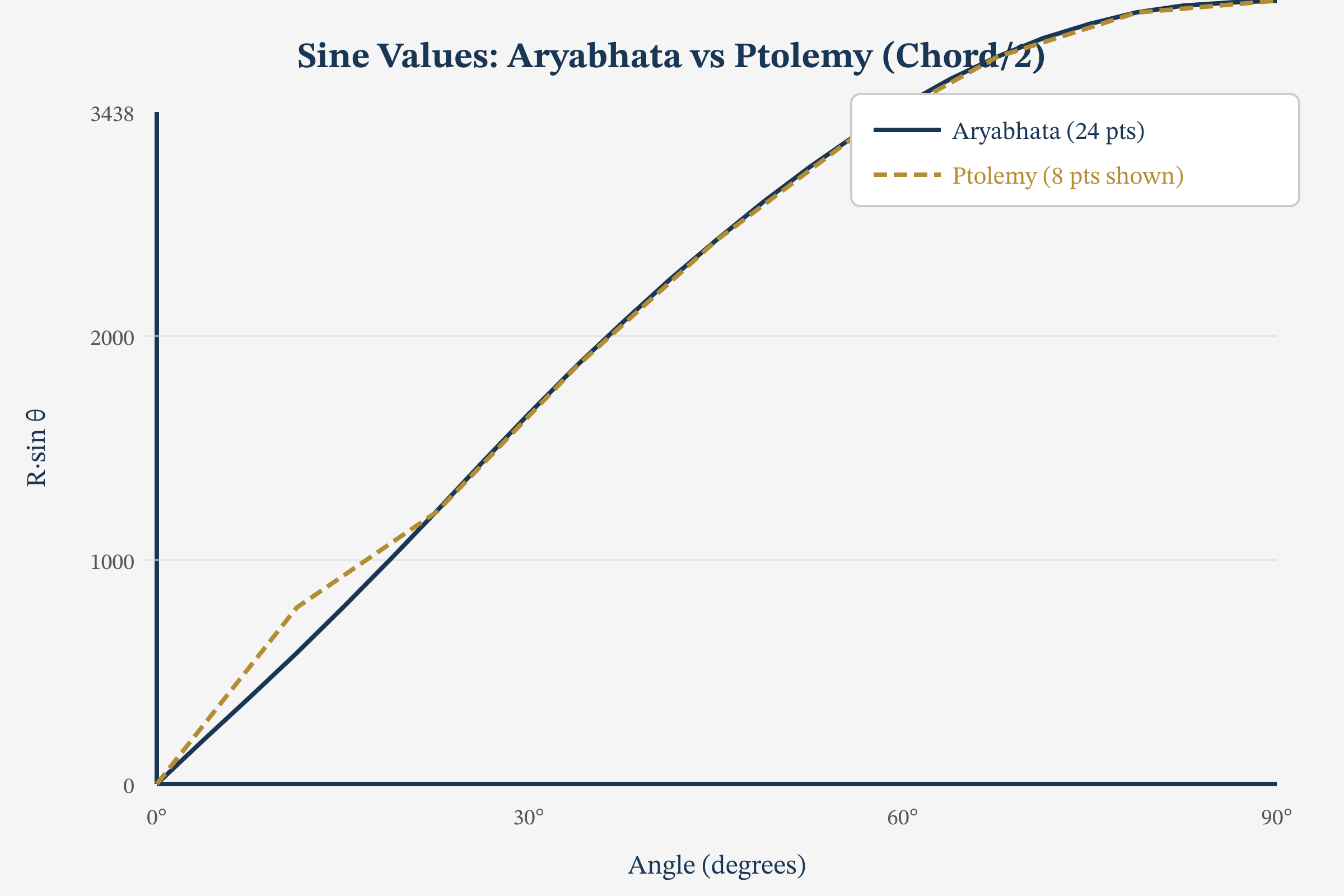
Comparison with Ptolemy’s Chord Table
Claudius Ptolemy (c. 150 CE) computed a table of chords in his Almagest. The relationship between chords and sines is:
$$ \text{chord}(\theta) = 2R\sin\!\left(\frac{\theta}{2}\right). $$
| Feature | Ptolemy (c. 150 CE) | Aryabhata (499 CE) |
|---|---|---|
| Function | Chord | Half-chord (sine) |
| Radius | 60 | 3438 |
| Increment | 0.5° | 3.75° |
| Entries | 360 | 24 |
| Method | Geometric (Ptolemy’s theorem) | Difference equation |
Remark. Although Ptolemy’s table is finer-grained, Aryabhata’s innovation is conceptual: the shift from chords to half-chords (sines) is fundamental, and the recursive computational method via a difference equation is more amenable to systematic calculation and theoretical generalisation.
Astronomy and Planetary Models
Earth’s Rotation
A Revolutionary Claim. Aryabhata asserted that the apparent daily rotation of the heavens is actually caused by the Earth spinning on its axis. In Golapada 9, he writes:
“Just as a man in a boat moving forward sees the stationary objects [on the shore] as moving backward, just so are the stationary stars seen by the people at Lanka [on the equator] as moving exactly towards the west.”
This is a clear statement of Earth’s axial rotation, made in the 5th century. Copernicus would not publish De Revolutionibus until 1543.
Remark 5.1. This claim was controversial even in India. Brahmagupta (628 CE) explicitly rejected it, arguing on physical grounds that objects would fly off a spinning Earth. The debate mirrors the later European resistance to Copernicanism.
The Sidereal Year
Theorem 5.1 (Aryabhata’s Sidereal Year). Aryabhata computed the length of the sidereal year as:
$$ Y = 365 \text{ days},\; 6 \text{ hours},\; 12 \text{ minutes},\; 30 \text{ seconds} = 365.25858\overline{3} \text{ days}. $$
The modern value is \(365.25636\) days. The error is:
$$ |365.25858 – 365.25636| = 0.00222 \text{ days} \approx 3 \text{ minutes } 12 \text{ seconds}. $$
Remark. An error of roughly 3 minutes in a year-long period, measured with naked-eye astronomy and water clocks, is an achievement of extraordinary precision.
Eclipse Calculations
Aryabhata gave a correct physical explanation of eclipses: the Moon’s shadow falls on Earth (solar eclipse), and Earth’s shadow falls on the Moon (lunar eclipse). This was a departure from the mythological Rahu-Ketu explanation prevalent in popular culture, though the Rahu concept was already being reinterpreted astronomically.
Definition 5.1 (Eclipse Condition). A lunar eclipse occurs when the Moon is near a node of its orbit (intersection with the ecliptic) at full moon:
$$ |\beta| < \frac{r_{\text{shadow}} + r_{\text{Moon}}}{d_{\text{Moon}}}, $$
where \(\beta\) is the lunar latitude, \(r_{\text{shadow}}\) is the radius of Earth’s shadow cone at the Moon’s distance, \(r_{\text{Moon}}\) is the Moon’s radius, and \(d_{\text{Moon}}\) is the Earth-Moon distance.
Planetary Models
Aryabhata used an epicyclic model for planetary motion, similar in structure to Ptolemy’s but with different parameters. Each planet moves on a small circle (epicycle) whose centre moves on a larger circle (deferent) centred on Earth.
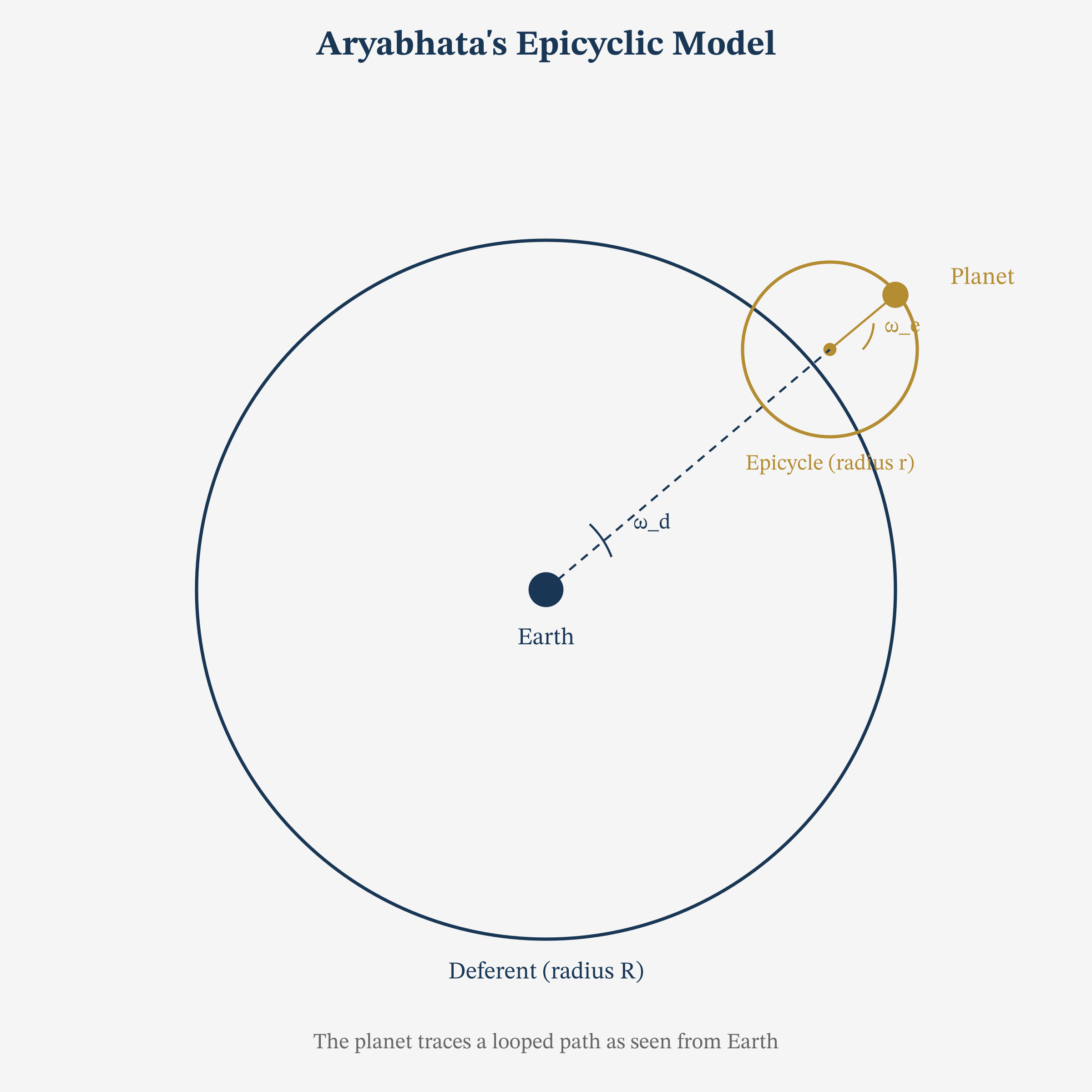
Proposition 5.2 (Epicycle-Eccentric Equivalence). The epicyclic model with epicycle radius \(r\) on a deferent of radius \(R\) produces the same apparent motion as an eccentric circle of radius \(R\) with centre offset by \(r\) from the observer, provided the angular velocities are appropriately matched.
Proof. Let the deferent centre be at the origin, and the observer at \(O\). In the epicyclic model, the planet’s position is:
$$ P = R e^{i\omega_d t} + r e^{i\omega_e t}, $$
where \(\omega_d\) and \(\omega_e\) are the deferent and epicyclic angular velocities. Setting \(\omega_e = -\omega_d\) (the case of the Sun), we get:
$$ P = R e^{i\omega_d t} + r e^{-i\omega_d t}. $$
More directly, if we write \(P = R e^{i\omega_d t} + r\) (fixed epicycle direction), then \(P\) traces a circle of radius \(R\) centred at \((r, 0)\), which is an eccentric model with eccentricity \(r\). ∎
| Body | Aryabhata (days) | Modern (days) | Error |
|---|---|---|---|
| Moon (sidereal) | 27.3217 | 27.3217 | < 0.001% |
| Mercury | 87.97 | 87.969 | ~0.001% |
| Venus | 224.70 | 224.701 | < 0.001% |
| Mars | 686.98 | 686.971 | ~0.001% |
| Jupiter | 4332.27 | 4332.59 | ~0.007% |
| Saturn | 10766.07 | 10759.22 | ~0.06% |
The Kuttaka Method in Detail
The kuttaka (“pulverizer”) is Aryabhata’s algorithm for solving linear indeterminate equations. It is equivalent to the extended Euclidean algorithm and intimately connected to continued fractions.
The Problem
Definition 6.1 (Linear Indeterminate Equation). Given integers \(a, b > 0\) and \(c\) with \(\gcd(a, b) \mid c\), find integers \(x, y\) satisfying:
$$ ax – by = c. $$
Theorem 6.1 (Existence and Structure of Solutions). The equation \(ax – by = c\) has integer solutions if and only if \(\gcd(a, b) \mid c\). If \((x_0, y_0)\) is one solution, then all solutions are given by:
$$ x = x_0 + \frac{b}{\gcd(a,b)}\,t, \quad y = y_0 + \frac{a}{\gcd(a,b)}\,t, \quad t \in ℤ. $$
Proof. Necessity. If \(ax – by = c\) and \(d = \gcd(a,b)\), then \(d \mid ax\) and \(d \mid by\), so \(d \mid c\).
Existence. By Bézout’s identity, there exist \(u, v \in ℤ\) with \(au + bv = d\). Then \(x_0 = uc/d\), \(y_0 = -vc/d\) satisfy \(ax_0 – by_0 = c\).
General solution. If \((x_0, y_0)\) and \((x_1, y_1)\) are both solutions, then \(a(x_1 – x_0) = b(y_1 – y_0)\). Dividing by \(d\): \((a/d)(x_1 – x_0) = (b/d)(y_1 – y_0)\). Since \(\gcd(a/d, b/d) = 1\), we need \((b/d) \mid (x_1 – x_0)\), giving the stated parametrisation. ∎
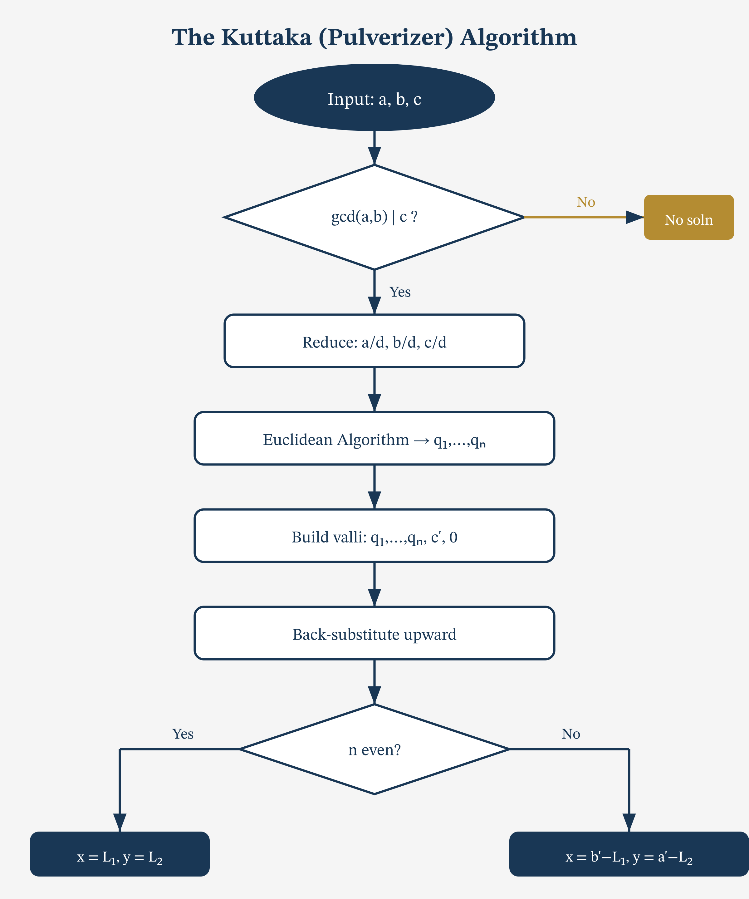
The Kuttaka Algorithm
Definition 6.2 (The Kuttaka (Pulverizer) Algorithm). To solve \(ax \equiv c \pmod{b}\) (equivalently, find \(x, y\) with \(ax – by = c\)):
- Step 1. Without loss of generality, ensure \(a > b\) (otherwise swap and adjust at the end). Set \(d = \gcd(a, b)\); if \(d \nmid c\), no solution exists. Otherwise, divide through by \(d\) to get \(a’x – b’y = c’\) with \(\gcd(a’, b’) = 1\).
- Step 2. Perform the Euclidean algorithm on \(a’\) and \(b’\), recording the sequence of quotients \(q_1, q_2, \ldots, q_n\): $$ \begin{aligned} a’ &= q_1 b’ + r_1, \\ b’ &= q_2 r_1 + r_2, \\ r_1 &= q_3 r_2 + r_3, \\ &\;\;\vdots \\ r_{n-2} &= q_n r_{n-1} + 0. \end{aligned} $$
- Step 3. Set up the valli (column): write the quotients \(q_1, q_2, \ldots, q_n\) in a column, and append \(c’\) and \(0\) at the bottom.
- Step 4. Work upward: starting from the bottom, compute \(L_{n-1} = q_n \cdot c’ + 0 = q_n c’\), then \(L_{k} = q_{k+1} L_{k+1} + L_{k+2}\) until reaching the top.
- Step 5. If \(n\) is even, \(x = L_1\), \(y = L_2\). If \(n\) is odd, apply a sign correction: \(x = b’ – L_1\), \(y = a’ – L_2\).
Example 6.1 (Solving \(137x – 60y = 1\)). We solve \(137x – 60y = 1\) using the kuttaka.
Step 1. \(\gcd(137, 60) = 1 \mid 1\), so solutions exist.
Step 2. Euclidean algorithm:
$$ \begin{aligned} 137 &= 2 \cdot 60 + 17, \\ 60 &= 3 \cdot 17 + 9, \\ 17 &= 1 \cdot 9 + 8, \\ 9 &= 1 \cdot 8 + 1, \\ 8 &= 8 \cdot 1 + 0. \end{aligned} $$
Quotients: \(q_1 = 2,\; q_2 = 3,\; q_3 = 1,\; q_4 = 1,\; q_5 = 8\).
Step 3. Valli column (top to bottom): \(2, 3, 1, 1, 8, c’=1, 0\).
Step 4. Work upward:
$$ \begin{aligned} L_5 &= 8 \cdot 1 + 0 = 8, \\ L_4 &= 1 \cdot 8 + 1 = 9, \\ L_3 &= 1 \cdot 9 + 8 = 17, \\ L_2 &= 3 \cdot 17 + 9 = 60, \\ L_1 &= 2 \cdot 60 + 17 = 137. \end{aligned} $$
Step 5. Using the extended Euclidean algorithm back-substitution:
$$ \begin{aligned} 1 &= 9 – 1 \cdot 8 \\ &= 9 – 1(17 – 1 \cdot 9) = 2 \cdot 9 – 17 \\ &= 2(60 – 3 \cdot 17) – 17 = 2 \cdot 60 – 7 \cdot 17 \\ &= 2 \cdot 60 – 7(137 – 2 \cdot 60) = 16 \cdot 60 – 7 \cdot 137. \end{aligned} $$
So \(137(-7) – 60(-16) = -959 + 960 = 1\), giving \(x = -7, y = -16\). For positive solutions: \(x = -7 + 60 = 53\), \(y = -16 + 137 = 121\). Check: \(137 \times 53 – 60 \times 121 = 7261 – 7260 = 1\). ✓
Example 6.2 (Astronomical Application: Solving \(576x – 210y = 6\)). This type of equation arises when computing the ahargana (day-count) in Indian astronomy.
Step 1. \(\gcd(576, 210) = 6 \mid 6\). Divide by 6: \(96x – 35y = 1\).
Step 2. Euclidean algorithm:
$$ \begin{aligned} 96 &= 2 \cdot 35 + 26, \\ 35 &= 1 \cdot 26 + 9, \\ 26 &= 2 \cdot 9 + 8, \\ 9 &= 1 \cdot 8 + 1. \end{aligned} $$
Back-substitution:
$$ \begin{aligned} 1 &= 9 – 1 \cdot 8 = 9 – (26 – 2 \cdot 9) = 3 \cdot 9 – 26 \\ &= 3(35 – 26) – 26 = 3 \cdot 35 – 4 \cdot 26 \\ &= 3 \cdot 35 – 4(96 – 2 \cdot 35) = 11 \cdot 35 – 4 \cdot 96. \end{aligned} $$
So \(96(-4) – 35(-11) = -384 + 385 = 1\), giving \(x_0 = -4\), \(y_0 = -11\). Positive solution: \(x = -4 + 35 = 31\), \(y = -11 + 96 = 85\). Check: \(96 \times 31 – 35 \times 85 = 2976 – 2975 = 1\). ✓
For the original equation: \(576 \times 31 – 210 \times 85 = 17856 – 17850 = 6\). ✓
Connection to Continued Fractions
Theorem 6.2 (Kuttaka and Continued Fractions). The quotients \(q_1, q_2, \ldots, q_n\) in the kuttaka algorithm are exactly the partial quotients of the continued fraction expansion:
$$ \frac{a}{b} = q_1 + \cfrac{1}{q_2 + \cfrac{1}{q_3 + \cfrac{1}{\ddots + \cfrac{1}{q_n}}}}. $$
The convergents \(p_k/q_k\) of this continued fraction satisfy \(|ap_k – bq_k| = 1\) when \(\gcd(a,b) = 1\) and \(k = n-1\).
Proof. This follows from the well-known theory of continued fractions: the convergents \(h_k/k_k\) satisfy the recurrence \(h_k = q_k h_{k-1} + h_{k-2}\), \(k_k = q_k k_{k-1} + k_{k-2}\), with \(h_k k_{k-1} – h_{k-1} k_k = (-1)^k\). The kuttaka’s upward computation is precisely this recurrence read backward. ∎
Modern Interpretation: Modular Arithmetic
Corollary: The equation \(ax \equiv c \pmod{b}\) is solvable if and only if \(\gcd(a,b) \mid c\). When \(\gcd(a,b) = 1\), the solution is unique modulo \(b\) and can be found by the kuttaka/extended Euclidean algorithm.
Remark: The kuttaka is thus equivalent to computing modular inverses. In modern cryptography (RSA, Diffie-Hellman), modular inverses are computed billions of times per second worldwide. Each such computation follows, in essence, Aryabhata’s 1500-year-old algorithm.
The Kuttaka in Modern Terms. Aryabhata’s kuttaka algorithm is:
- The extended Euclidean algorithm for \(\gcd\) and Bézout coefficients.
- Equivalent to computing convergents of continued fractions.
- The standard method for modular inversion in number theory and cryptography.
It is a testament to Aryabhata’s genius that an algorithm devised for astronomical calculations in the 5th century remains a cornerstone of 21st-century computer science.
Legacy and Transmission
Bhaskara I’s Commentary
Bhaskara I (c. 600-680 CE) wrote the earliest surviving commentary on the Aryabhatiya in 629 CE, the Aryabhatiyabhashya. His work is invaluable because:
- It clarifies the terse, versified formulas of the original.
- It provides worked examples that illuminate Aryabhata’s methods.
- It contains Bhaskara I’s own remarkable rational approximation for the sine function: $$ \sin\theta \approx \frac{16\theta(\pi – \theta)}{5\pi^2 – 4\theta(\pi – \theta)}, \quad 0 \leq \theta \leq \pi. $$
Example 7.1 (Testing Bhaskara I’s Sine Approximation). At \(\theta = \pi/6\) (i.e., \(30°\)):
$$ \begin{aligned} \sin(\pi/6) &= 0.5, \\ \text{Approx} &= \frac{16 \cdot \frac{\pi}{6} \cdot \frac{5\pi}{6}}{5\pi^2 – 4 \cdot \frac{\pi}{6} \cdot \frac{5\pi}{6}} = \frac{16 \cdot \frac{5\pi^2}{36}}{5\pi^2 – \frac{20\pi^2}{36}} = \frac{\frac{80\pi^2}{36}}{\frac{160\pi^2}{36}} = \frac{80}{160} = 0.5. \end{aligned} $$
Exact! At \(\theta = \pi/4\) (\(45°\)):
$$ \text{Approx} = \frac{16 \cdot \frac{\pi}{4} \cdot \frac{3\pi}{4}}{5\pi^2 – 4 \cdot \frac{3\pi^2}{16}} = \frac{16 \cdot \frac{3\pi^2}{16}}{5\pi^2 – \frac{3\pi^2}{4}} = \frac{3\pi^2}{\frac{17\pi^2}{4}} = \frac{12}{17} \approx 0.70588. $$
Actual: \(\sin 45° \approx 0.70711\). Error: \(0.17\%\). Remarkably accurate for such a simple formula.
Influence on Later Indian Mathematicians
Aryabhata’s influence pervades all subsequent Indian mathematics:
- Brahmagupta (628 CE) built on Aryabhata’s kuttaka method, extending it to quadratic indeterminate equations (varga-prakriti: \(Nx^2 + 1 = y^2\)).
- Mahavira (c. 850 CE) expanded the combinatorial aspects.
- Bhaskara II (1150 CE) perfected the algorithmic tradition in the Lilavati and Bijaganita, always acknowledging the debt to Aryabhata.
- Madhava of Sangamagrama (c. 1340-1425) and the Kerala school extended Aryabhata’s trigonometric programme to infinite series: $$ \frac{\pi}{4} = 1 – \frac{1}{3} + \frac{1}{5} – \frac{1}{7} + \cdots $$ and the Taylor series for \(\sin\) and \(\cos\) – anticipating Gregory, Leibniz, and Newton by over two centuries.
Transmission to the Islamic World
Indian mathematical and astronomical texts were transmitted to the Islamic world through multiple channels:
- The Sindhind tradition: Indian astronomical texts (including methods from the Aryabhata school) were translated into Arabic in Baghdad under the Abbasid caliphs (8th-9th century).
- Al-Khwarizmi’s Zij al-Sindhind (c. 820) drew directly on Indian sources for its sine tables and computational methods.
- The Indian decimal numeral system, transmitted through Arabic scholars, became the “Hindu-Arabic” numerals now used worldwide.
Remark 7.1. Al-Biruni (973-1048), who spent years in India and wrote the encyclopaedic Tarikh al-Hind, provides our most detailed external account of Indian mathematical astronomy, including extensive discussion of Aryabhata’s methods.
Modern Recognition
- Aryabhata satellite (1975): India’s first satellite, launched by ISRO on 19 April 1975, was named after Aryabhata – a fitting tribute for the man who first correctly explained eclipses and computed planetary periods to extraordinary precision.
- Aryabhata Research Institute of Observational Sciences (ARIES): The premier Indian observatory at Nainital bears his name.
- The lunar crater Aryabhata on the Moon’s far side.
- The asteroid 4758 Aryabhata.
What Was Lost
Aryabhata is known to have written at least one other work, sometimes called the Aryabhata Siddhanta, which survives only in fragments quoted by later authors (notably Brahmagupta and Bhaskara I). The loss of this text – and likely others – means that our picture of Aryabhata’s mathematical knowledge is almost certainly incomplete.
Aryabhata’s Enduring Legacy. In 121 verses, Aryabhata:
- Established the sine function and constructed a systematic sine table.
- Invented the kuttaka algorithm (= extended Euclidean algorithm).
- Gave summation formulas for \(\sum k\), \(\sum k^2\), \(\sum k^3\).
- Approximated \(\pi\) to four decimal places.
- Asserted Earth’s axial rotation.
- Computed the sidereal year to within 3 minutes.
- Correctly explained solar and lunar eclipses.
All this at the age of 23. The Aryabhatiya is one of the most remarkable scientific documents in human history.
“Like the Sun, which gives light to all, Aryabhata illuminated the world with his knowledge.”
Bhaskara I, Aryabhatiyabhashya (629 CE)
Appendix A: Aryabhata’s Sine Differences
For reference, we list the complete sequence of 24 sine differences \(D_k\) as given in the Gitikapada:
| \(k\) | Angle | jya\((kh)\) | \(D_k\) | Second diff. \(\Delta^2\) |
|---|---|---|---|---|
| 1 | 3°45′ | 225 | 225 | – |
| 2 | 7°30′ | 449 | 224 | -1 |
| 3 | 11°15′ | 671 | 222 | -2 |
| 4 | 15°00′ | 890 | 219 | -3 |
| 5 | 18°45′ | 1105 | 215 | -4 |
| 6 | 22°30′ | 1315 | 210 | -5 |
| 7 | 26°15′ | 1520 | 205 | -5 |
| 8 | 30°00′ | 1719 | 199 | -6 |
| 9 | 33°45′ | 1910 | 191 | -8 |
| 10 | 37°30′ | 2093 | 183 | -8 |
| 11 | 41°15′ | 2267 | 174 | -9 |
| 12 | 45°00′ | 2431 | 164 | -10 |
| 13 | 48°45′ | 2585 | 154 | -10 |
| 14 | 52°30′ | 2728 | 143 | -11 |
| 15 | 56°15′ | 2859 | 131 | -12 |
| 16 | 60°00′ | 2978 | 119 | -12 |
| 17 | 63°45′ | 3084 | 106 | -13 |
| 18 | 67°30′ | 3177 | 93 | -13 |
| 19 | 71°15′ | 3256 | 79 | -14 |
| 20 | 75°00′ | 3321 | 65 | -14 |
| 21 | 78°45′ | 3372 | 51 | -14 |
| 22 | 82°30′ | 3409 | 37 | -14 |
| 23 | 86°15′ | 3431 | 22 | -15 |
| 24 | 90°00′ | 3438 | 7 | -15 |
Remark A.1. The second differences are approximately proportional to the sine values themselves, confirming Aryabhata’s recurrence relation (Theorem 4.1). The near-constancy of the second differences near \(90°\) reflects the fact that \(\sin\theta \approx 1\) and \(\sin”(\theta) = -\sin\theta \approx -1\) in that region.
Appendix B: The Kuttaka Algorithm – Flowchart Description
For implementation, the kuttaka algorithm can be expressed as follows:
- Input: \(a, b, c \in ℤ\) with \(a, b > 0\).
- Check: Compute \(d = \gcd(a, b)\). If \(d \nmid c\), output “No solution” and halt.
- Reduce: \(a \leftarrow a/d\), \(b \leftarrow b/d\), \(c \leftarrow c/d\).
- Initialise: \(r_0 = a\), \(r_1 = b\), \(s_0 = 1\), \(s_1 = 0\), \(t_0 = 0\), \(t_1 = 1\).
- Loop: While \(r_1 \neq 0\):
- \(q = \lfloor r_0 / r_1 \rfloor\).
- \((r_0, r_1) \leftarrow (r_1, r_0 – q \cdot r_1)\).
- \((s_0, s_1) \leftarrow (s_1, s_0 – q \cdot s_1)\).
- \((t_0, t_1) \leftarrow (t_1, t_0 – q \cdot t_1)\).
- Output: \(x = s_0 \cdot c\), \(y = -t_0 \cdot c\). Adjust to positive values modulo \(b\) and \(a\) respectively.
This is precisely the extended Euclidean algorithm, which Aryabhata discovered independently of (and possibly before) any comparable development in the Western mathematical tradition.