Variance and Standard Deviation

Variance and standard deviation measure how spread out values are around their mean. Two datasets can share the same average and look completely different in practice — one tightly clustered, one wildly scattered. Variance and standard deviation give you the number that captures the difference.

If you’ve ever compared two investments with the same expected return, two restaurants with the same average review, or two A/B test variants with the same mean lift, you’ve already needed this. Variance is the engine. Standard deviation is the version you actually report, in the same units as the data.

This study note covers the formulas (population vs sample), worked examples, the coefficient of variation, why we square deviations in the first place, the empirical rule, common mistakes that mislead even trained analysts, and the way variance plugs into the rest of statistics.

The Formulas

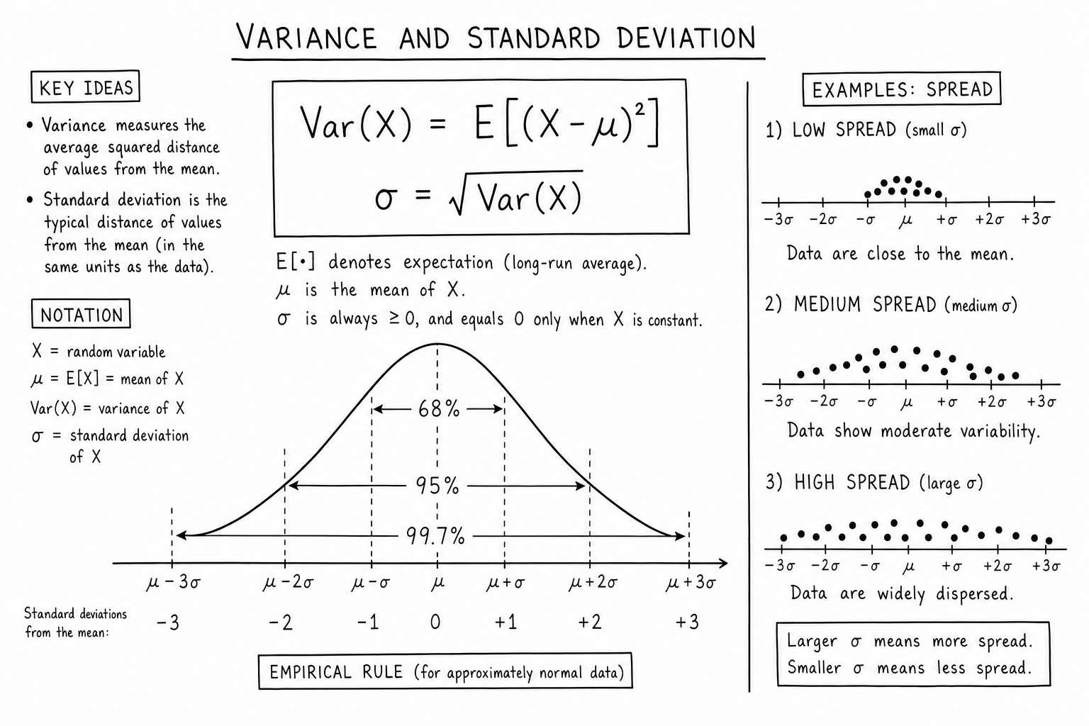
For a random variable \(X\) with mean \(\mu\):

$$\text{Var}(X) = E[(X – \mu)^2] = \sum_{i=1}^{n} p_i (x_i – \mu)^2$$ $$\sigma = \sqrt{\text{Var}(X)}$$

Variance is the average squared distance from the mean. Squaring punishes large deviations more than small ones and conveniently strips negative signs. Standard deviation \(\sigma\) is the square root, which puts the answer back in the original units.

For a sample (rather than the full population) of size \(n\), divide by \(n – 1\) instead of \(n\). This is Bessel’s correction:

$$s^2 = \frac{1}{n-1} \sum_{i=1}^{n} (x_i – \bar{x})^2$$

Bessel’s correction matters because the sample mean is closer to the sample data than the unknown population mean is. Dividing by \(n – 1\) corrects the bias and gives an unbiased estimator of population variance.

Worked Example: Two Investments, Same Mean

Two investments, each requiring 10,000 dollars upfront:

• A: 50% chance of returning 12,000 (+2,000 dollars), 50% chance of returning 8,000 (-2,000 dollars).
• B: 50% chance of returning 20,000 (+10,000 dollars), 50% chance of returning 0 (-10,000 dollars).

Both have \(E = 10{,}000\). The standard deviations diverge:

$$\sigma_A = \sqrt{0.5 \times 2{,}000^2 + 0.5 \times 2{,}000^2} = 2{,}000$$ $$\sigma_B = \sqrt{0.5 \times 10{,}000^2 + 0.5 \times 10{,}000^2} = 10{,}000$$

Investment B has 5× the spread for the same expected return. Same average, very different risk profile. Investment A wins unless you specifically need the upside that B’s variance brings.

This is why two stocks with identical historical mean returns can have wildly different risk-adjusted attractiveness, and why annualized volatility (essentially standard deviation of returns) is the headline risk metric in finance.

Worked Example: Quality Control

A factory produces 10mm bolts. Two production lines both target 10mm with the same average output:

• Line A: mean 10.00 mm, σ = 0.01 mm.
• Line B: mean 10.00 mm, σ = 0.05 mm.

If the spec calls for bolts within ±0.03 mm, Line A produces nearly perfect output (3σ tolerance), while Line B sees roughly 55% of bolts in spec (less than 1σ tolerance) and 45% scrap. Same mean, very different defect rate. Six Sigma quality programs are built around managing variance, not just mean — they target σ small enough that ±6σ still fits inside the spec window.

Coefficient of Variation

Standard deviation by itself doesn’t compare across scales. A 1,000 dollar standard deviation matters more around a 5,000 dollar mean than around a 100,000 dollar mean. The fix is the coefficient of variation:

$$CV = \frac{\sigma}{\mu}$$

CV expresses risk per unit of return. Use it to compare investments, projects, or processes that operate at different scales. Lower CV is generally better for the same kind of activity.

Coefficient of variation is also the natural metric for comparing distributions across units (lab measurements in different scales, customer wait times across different store sizes, click-through rates across vastly different traffic levels). It’s dimensionless, which makes cross-domain comparison meaningful.

Why Squared and Then Rooted?

You could measure spread with the average absolute deviation. Mathematicians prefer squaring because it makes the algebra cleaner: variances of independent random variables add, derivatives are smooth, and the normal distribution falls out of the math naturally.

The cost: variance reports squared units (squared dollars, squared seconds), which feels weird. That’s why you almost always report standard deviation in practice. Variance lives in the calculations; standard deviation lives in the conclusions.

Mean absolute deviation (MAD) is a perfectly valid alternative measure of spread and is more robust to outliers. It hasn’t won as the default because it doesn’t combine cleanly under operations like adding random variables, doesn’t yield a clean derivative, and doesn’t connect to the normal distribution the way variance does. Statistical theory grew around variance, so the tooling and convention reinforce it.

The Empirical Rule (68-95-99.7)

For approximately normal distributions:

• About 68% of values fall within ±1σ of the mean.
• About 95% fall within ±2σ.
• About 99.7% fall within ±3σ.

These three numbers are worth memorizing. They turn any mean and standard deviation into instant range estimates. They’re also the foundation for confidence intervals, z-scores, and quality-control limits.

The empirical rule fails for skewed and heavy-tailed distributions. Stock returns, network traffic, and earthquake magnitudes routinely produce 4σ and 5σ events that the normal-distribution version would call essentially impossible. Read more in the companion normal distribution note.

Properties That Make Variance Useful

• Constants drop out: \(\text{Var}(X + c) = \text{Var}(X)\). Adding a constant shifts the mean but not the spread.
• Constants scale quadratically: \(\text{Var}(cX) = c^2 \text{Var}(X)\). Standard deviation scales linearly: \(\sigma(cX) = |c| \cdot \sigma(X)\).
• Independent variables add: \(\text{Var}(X + Y) = \text{Var}(X) + \text{Var}(Y)\). This is why standard deviations don’t add but variances do; it’s the basis for portfolio risk math, error propagation, and analysis of variance.
• Sample mean variance: \(\text{Var}(\bar{X}) = \sigma^2 / n\). Bigger samples shrink sampling variance proportionally to \(n\); standard error shrinks with \(\sqrt{n}\). This is the central reason larger surveys give tighter estimates.

Where Variance Shows Up

• Investing. Volatility is just standard deviation of returns. The Sharpe ratio is excess return divided by standard deviation. Read more in the mathematics of risk assessment.
• Quality control. Six Sigma processes target a defect rate so low that the spec limits sit six standard deviations away from the mean.
• Forecasting. Confidence intervals are built from standard deviation. Reporting a forecast as 100,000 ± 15,000 communicates the uncertainty.
• Business statistics. Variance underlies regression, ANOVA, and almost every test in business statistics.
• Machine learning. Bias-variance tradeoff is the central concept in supervised learning: high-variance models overfit; high-bias models underfit. The whole regularization toolkit (ridge, lasso, dropout, early stopping) is variance management.
• Genetics and biology. Heritability is defined as the proportion of phenotype variance attributable to genetic variance.

Common Mistakes

1. Confusing population and sample formulas. Use \(n – 1\) for samples. Most spreadsheet functions (e.g., STDEV.S vs STDEV.P in Excel, var() vs var(ddof=0) in pandas) ask which one you want; pick deliberately.
2. Forgetting that variance and standard deviation are sensitive to outliers. One extreme value can shift them dramatically. For data with heavy outliers, consider robust alternatives like median absolute deviation or interquartile range.
3. Reporting variance instead of standard deviation. Variance is in squared units and rarely intuitive to a non-statistical audience. Convert to standard deviation for any report intended to communicate risk or spread.
4. Assuming constant variance. Real-world data often has variance that depends on the level of the variable (heteroskedasticity). Linear regression and many other classical methods assume constant variance, and violations distort inference.
5. Adding standard deviations. Standard deviations don’t add. Variances do (for independent variables), and you take the square root at the end. Most “rule of thumb” addition errors come from forgetting this.

Variance Decomposition (ANOVA)

Analysis of Variance (ANOVA) decomposes total variance in a dataset into components attributable to different sources. Total sum of squares = between-group sum of squares + within-group sum of squares. The F-statistic ratios between-group variance to within-group variance to test whether group means differ significantly.

ANOVA is the workhorse of experimental design across psychology, agriculture, biology, and manufacturing. Two-way ANOVA, repeated-measures ANOVA, MANOVA — all variants of the same idea: split variance into interpretable buckets and test which buckets matter.

Variance in Portfolio Theory

Modern Portfolio Theory (Markowitz, 1952) treats portfolio variance as the central risk measure. The variance of a portfolio of two assets is:

$$\sigma_p^2 = w_1^2 \sigma_1^2 + w_2^2 \sigma_2^2 + 2 w_1 w_2 \rho_{12} \sigma_1 \sigma_2$$

where \(w_i\) are weights and \(\rho_{12}\) is the correlation. The third term is the magic: when correlations are low or negative, portfolio variance can be lower than the variance of either individual asset. This is the formal basis of diversification.

The efficient frontier — the set of portfolios with maximum return for each level of variance — falls out of solving a quadratic optimization on this variance formula. Most quantitative investing builds on top of this framework.

Robust Alternatives to Variance

Variance is sensitive to outliers because deviations are squared. For data with heavy tails or contamination, robust alternatives perform better:

• Median absolute deviation (MAD): the median of \(|x_i – \text{median}(x)|\). Resistant to outliers and easy to compute.
• Interquartile range (IQR): the difference between the 75th and 25th percentiles. Used in box plots and outlier flagging.
• Trimmed variance: compute variance after removing extreme percentiles (e.g., trim top and bottom 5%).
• Winsorized variance: replace extreme values with the boundary percentiles before computing variance.

For analyses where outliers are real and relevant (financial risk, extreme weather), use heavy-tailed distributions instead of trying to robustify variance.

Sample Variance and Degrees of Freedom

The \(n – 1\) in the sample variance formula represents degrees of freedom. With \(n\) data points and one estimated parameter (the sample mean), only \(n – 1\) of the deviations are free to vary; the last one is determined by the constraint that deviations sum to zero.

Degrees of freedom show up everywhere in classical statistics. Chi-squared tests, t-tests, F-tests, and ANOVA all use degrees of freedom to compute the right reference distribution. Confidence intervals for the mean use \(t_{n-1}\) precisely because variance was estimated from the same sample.

For complex models with many parameters (regression with k predictors), the residual variance uses \(n – k – 1\) degrees of freedom. Each estimated parameter eats one degree of freedom from the residual variance estimate.

Variance in A/B Testing

The variance of the difference between two sample means is the sum of their individual variances (since groups are independent). Standard error of the difference:

$$SE_{\text{diff}} = \sqrt{\frac{\sigma_A^2}{n_A} + \frac{\sigma_B^2}{n_B}}$$

This standard error feeds the z-score or t-score that A/B test calculators use to compute p-values and confidence intervals. The variance of conversion rate differences depends on the rates themselves: \(\sigma^2 \approx p(1-p)\) for proportions. That’s why A/B testing dashboards report results with margins of error that shrink with sample size at rate \(\sqrt{n}\).

Variance Inflation Factor in Regression

When predictors in a regression are correlated (multicollinearity), the variance of regression coefficient estimates inflates. The Variance Inflation Factor (VIF) quantifies this:

$$\text{VIF}_j = \frac{1}{1 – R_j^2}$$

where \(R_j^2\) is the R-squared from regressing predictor \(j\) on all other predictors. VIF > 5 suggests problematic multicollinearity; VIF > 10 is usually treated as serious. The fix is dropping correlated predictors, combining them, or switching to regularized regression (ridge, lasso) that handles multicollinearity gracefully.

Variance and Statistical Power

The probability of detecting a real effect in an experiment (statistical power) depends on three things: effect size, sample size, and variance. High variance reduces power; low variance increases it. Power calculations use this relationship to determine the sample size needed to detect a given effect with a given probability.

This is why pre-experiment power analysis matters: running an underpowered study against high-variance data wastes resources and produces inconclusive results. Pilot studies are often run specifically to estimate the variance, which then feeds the power calculation for the main experiment.

How to Reduce Variance in Practice

Three reliable ways to reduce variance in any process or measurement: increase sample size (variance of the mean shrinks at rate 1/n), tighten the inputs (lower input variance produces lower output variance), or average multiple independent measurements (averaging k independent estimates divides variance by k). All three are everyday tools in experimental design, manufacturing, and analytics.

Variance reduction is also why ensemble methods in machine learning (bagging, random forests) outperform single models — they average independent predictions, cutting variance without hurting bias much. The same logic applies to averaging multiple sensor readings, running replicate experiments, or pooling data across similar studies in a meta-analysis.

Worked Example: Standard Deviation of Returns

Suppose a stock had monthly returns over the past year of: 2%, −1%, 3%, 5%, −2%, 0%, 4%, −3%, 6%, 1%, 2%, −1%. Mean return ≈ 1.33%. Squared deviations sum to about 91. Sample variance = 91 / 11 ≈ 8.27. Standard deviation = √8.27 ≈ 2.88%.

Annualized volatility = monthly σ × √12 ≈ 9.97%. That’s the headline volatility figure for this stock over the period. Compare to a typical broad-market index volatility (15–20% annually) or a bond fund (3–6%) and you can immediately rank the risk profile.

The √12 scaling assumes returns are independent month to month — usually a reasonable approximation for short windows but breaks down for long horizons where mean reversion or trend matters.

Variance vs Range: Why Range Isn’t Enough

Range — the difference between the maximum and minimum value — is the simplest measure of spread. It tells you how wide the data is but ignores everything in between. Two datasets can have the same range and very different distributions.

Consider [0, 1, 1, 1, 1, 1, 1, 1, 1, 10] vs [0, 1, 2, 3, 4, 5, 6, 7, 8, 10]. Both have range 10. The first has variance ≈ 8.5; the second has variance ≈ 11.0. Range hides this difference. Variance and standard deviation use every data point, weighted by their squared distance from the mean, and capture the underlying shape of the distribution.

Range is also extremely sensitive to outliers — a single extreme value sets the range, regardless of how dense the rest of the data is. Variance is sensitive too, but at least every point contributes proportionally.

FAQs