Definitions and Types of Integral Equations

In this article, I will explain what Integral Equations are, how they are structured and what are certain types of Integral Equations.

What is an Integral Equation?

An integral equation is an equation in which an unknown function appears under one or more integration signs.

Any integral calculus statement like — $y= \int_a^b \phi(x) dx$ can be considered as an integral equation.

If you noticed, I have used two integration limits (a and b) in the above integral equation – they are special in this discussion, and their significance will be discussed later in the article.

Linear Integral Equations

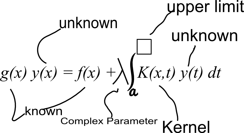
A general type of integral equation, $g(x) y(x) = f(x) + \lambda \int_a^\Box K(x, t) y(t) dt$ is called linear integral equation as only linear operations are performed in the equation.

The one, which is not linear, is obviously called a “Non-linear integral equation”.

We generally mean linear integral equation when we say integral equation. When a non-linear integral equation is to be called, it is called exclusively.

In the general type of the linear equation

$g(x) y(x) = f(x) + \lambda \int_a^\Box K(x, t) y(t) dt$

we have used a ‘box $\Box$’ to indicate the higher limit of the integration.

Types of Integral Equations

Integral Equations can be of two types according to whether the box $\Box$ (the upper limit) is a constant, $b$ or a variable, $x$.

The first type of integral equations which involve constants as both the limits — are called Fredholm Type Integral equations.

On the other hand, when one of the limits is a variable ($x$, the independent variable of which $y$, $f$ and $K$ are functions), such integral equations are called Volterra’s Integral Equations.

In an integral equation, $y$ is to be determined with $g$, $f$ and $K$ being known and $\lambda$ being a non-zero complex parameter. The function $K (x,t)$ is called the ‘kernel’ of the integral equation.

Structure of an Integral Equation

Types of Fredholm Integral Equations

As the general form of Fredholm Integral Equation is $g(x) y(x) = f(x) + \lambda \int_a^b K(x, t) y(t) dt$, there may be following other types of it according to the values of $g$ and $f$ :

1. Fredholm Integral Equation of First Kind  —when — $g(x) = 0$
   $f(x) + \lambda \int_a^b K(x, t) y(t) dt=0$
2. Fredholm Integral Equation of Second Kind  —when — $g(x) =1$
   $y(x) = f(x) + \lambda \int_a^b K(x, t) y(t) dt$
3. Fredholm Integral Equation of Homogeneous Second Kind —when $f(x)=0$
   and $g(x)=1$
   $y(x) = \lambda \int_a^b K(x, t) y(t) dt$
4. The general equation of Fredholm equation is also called Fredholm Equation of Third/Final kind, with $f(x) \neq 0, 1 \neq g(x)\neq 0$.

Types of Volterra Integral Equations

As the general form of Volterra Integral Equation is $g(x) y(x) = f(x) + \lambda \int_a^x K(x, t) y(t) dt$, there may be following other types of it according to the values of $g$ and $f$ :

1. Volterra Integral Equation of First Kind  —when — $g(x) = 0$
   $f(x) + \lambda \int_a^x K(x, t) y(t) dt=0$
2. Volterra Integral Equation of Second Kind  —when — $g(x) =1$
   $y(x) = f(x) + \lambda \int_a^x K(x, t) y(t) dt$
3. Volterra Integral Equation of Homogeneous Second Kind —when $f(x)=0$
   and $g(x)=1$
   $y(x) = \lambda \int_a^x K(x, t) y(t) dt$
4. The general equation of Volterra equation is also called the Volterra Equation of Third/Final kind, with $f(x) \neq 0, 1 \neq g(x)\neq 0$.

Singular Integral equations

In the general Fredholm/Volterra Integral equations, there arise two singular situations:

• the limit $a \to -\infty$ and $\Box \to \infty$.
• the kernel $K(x,t) = \pm \infty$ at some points in the integration limit $[a, \Box]$.

Then, such integral equations are called Singular (Linear) Integral Equations. Based on these two singular situations, here are two examples of the Singular Integral equations.

Kernels

The nature of the solution of integral equations solely depends on the nature of the Kernel of the integral equation K(x,t).

Kernels are of the following special types:

Symmetric Kernel

When the kernel $K(x,t)$ is symmetric or complex symmetric or Hermitian, if $K(x,t)= \bar{K}(t,x)$ .

Here bar  $\bar{K}(t,x)$ denotes the complex conjugate of $K(t,x)$.

That’s if there is no imaginary part of the kernel, then $K(x, t) = K(t, x)$ implies that $K$ is a symmetric kernel.

For example $K(x,t)= \sin (x+t)$ is symmetric kernel.

Separable or Degenerate Kernel

A kernel $K(x,t)$ is called separable if it can be expressed as the sum of a finite number of terms, each of which is the product of ‘a function’ of x only and ‘a function’ of t only, i.e., $K(x,t)= \displaystyle{\sum_{n=1}^{\infty}} \phi_i (x) \psi_i (t)$

Difference Kernel

When $K(x,t) = K(x-t)$, the kernel is called difference kernel.

Resolvent or Reciprocal Kernel

The solution of the integral equation $y(x) = f(x) + \lambda \int_a^\Box K(x, t) y(t) dt$ is of the form $y(x) = f(x) + \lambda \int_a^\Box \mathfrak{R}(x, t;\lambda) f(t) dt$.

The kernel $\mathfrak{R}(x, t;\lambda)$ of the solution is called resolvent or reciprocal kernel.

Integral Equations of Convolution Type

The integral equation $g(x) y(x) = f(x) + \lambda \int_a^\Box K(x, t) y(t) dt$ is called of integral equation of convolution type when the kernel $K(x,t)$ is difference kernel, i.e., $K(x,t) = K(x-t)$.

Let $y_1(x)$ and $y_2(x)$ be two continuous functions defined for $x \in E \subseteq\mathbb{R}$ then the convolution of $y_1$ and $y_2$ is given by

$$y_1 * y_2 = \int_E y_1 (x-t) y_2(t) dt$$

$$=\int_E y_2 (x-t) y_1(t) dt$$

For standard convolution, the limits are $-\infty$ and $\infty$.

Eigenvalues and Eigenfunctions of Integral Equations

The homogeneous integral equation $y(x) = \lambda \int_a^\Box K(x, t) y(t) dt$ has the obvious solution $y(x)=0$ which is called the zero solution or the trivial solution of the integral equation.

Except this, the values of $\lambda$ for which the integral equation has non-zero solution $y(x) \neq 0$, are called the eigenvalues of integral equation or eigenvalues of the kernel.

Every non-zero solution $y(x)\neq 0$ is called an eigenfunction corresponding to the obtained eigenvalue $\lambda$.

• Note that $\lambda \neq 0$
• If $y(x)$ an eigenfunction corresponding to eigenvalue $\lambda$ then $c \cdot y(x)$ is also an eigenfunction corresponding to $\lambda$

Leibnitz Rule of Differentiation under the integral sign

Let $F(x,t)$ and $\dfrac{\partial F}{\partial x}$ be continuous functions of both x and t and let the first derivatives of $G(x)$ and $H(x)$ are also continuous, then

$\dfrac{d}{dx} \displaystyle {\int_{G(x)}^{H(x)}} F(x,t) dt$

$= \displaystyle {\int_{G(x)}^{H(x)}}\dfrac{\partial F}{\partial x} dt + F(x, H(x)) \dfrac{dH}{dx} – \\ F(x, G(x)) \dfrac{dG}{dx}$.

This formula is called Leibnitz’s Rule of differentiation under integration sign. In a special case, when G(x) and H(x) both are absolute (constants) –let $G(x) =a$, $H(x)=b \iff dG/dx =0=dH/dx$ ; then

$\dfrac{d}{dx} \displaystyle {\int_a^b} F(x,t) dt = \displaystyle {\int_a^b}\dfrac{\partial F}{\partial x} dt$

Changing Integral Equation with Multiple Integrals into Standard Simple  Integral

(Multiple Integral Into Simple Integral — The magical formula)

Say, the integral of order n is given by $\displaystyle{\int_{\Delta}^{\Box}} f(x) dx^n$

We can prove that $\displaystyle{\int_{a}^{t}} f(x) dx^n = \displaystyle{\int_{a}^{t}} \dfrac{(t-x)^{n-1}}{(n-1)!} f(x) dx$