The Quadratic Formula

Q: Why does the quadratic formula always work?

Because it's derived from the universal technique of completing the square, which works on any quadratic equation. The formula encodes the full recipe in one expression, including the discriminant case structure for real, repeated, or complex roots.

Q: What does the discriminant tell me?

The discriminant b² − 4ac determines the nature of the roots. Positive: two distinct real roots. Zero: one repeated real root. Negative: two complex conjugate roots. Computing it first tells you what to expect before doing the full formula evaluation.

Q: When should I factor instead of using the formula?

When the quadratic has obvious integer roots, factoring is faster. Look for two numbers that multiply to c (or c/a) and add to b (or b/a). If you can't factor in 30 seconds, switch to the formula — it always works, even when factoring fails.

Q: Why is there a ± sign in the formula?

Because the square root produces both a positive and a negative value. The two values give two solutions, which are the two intersections of the parabola with the x-axis. Quadratics have exactly two roots (counted with multiplicity, over the complex numbers).

Q: Can the quadratic formula give complex solutions?

Yes — when the discriminant is negative, the square root produces an imaginary number, and the roots become complex conjugates of the form a ± bi. Complex roots are mathematically valid; they just don't correspond to x-axis intersections in real space.

Q: How do I know which form to use: standard, vertex, or factored?

Standard form is best for the formula and general manipulation. Vertex form is best for graphing and finding extrema. Factored form is best when roots are known. Practice converting between all three and switching based on what the problem needs.

Q: What is completing the square?

An algebraic technique that rewrites a quadratic ax² + bx + c as a(x − h)² + k. It's the derivation engine behind the quadratic formula and the standard way to convert standard form into vertex form. Worth practicing because it generalizes to many other algebra problems.

Q: Who discovered the quadratic formula?

Pieces of it date back to Babylonian mathematicians (~2000 BCE). Brahmagupta gave a complete general solution in 628 CE. Al-Khwarizmi systematized quadratic solving in the 9th century. The modern notation crystallized in the 16th and 17th centuries with Viète and Descartes.

Q: What is Vieta's formula for quadratics?

For roots r₁ and r₂ of ax² + bx + c = 0: sum r₁ + r₂ = −b/a, product r₁r₂ = c/a. These let you verify your solutions and sometimes find roots faster than the formula by inspection.

Q: How is the quadratic formula used in physics?

Projectile motion is the most common application. Position varies as ½gt², which gives a quadratic in time. Solving for landing time, time of flight, or intersection times all use the quadratic formula. Other uses include resonant frequency calculations and beam deflection analysis.

The quadratic formula solves every equation of the form $ax^2 + bx + c = 0$, no matter how messy the coefficients. It’s the closed-form solution to the second most important polynomial equation type in mathematics, and it’s the first formula most students memorize because it actually works on every problem in its class.

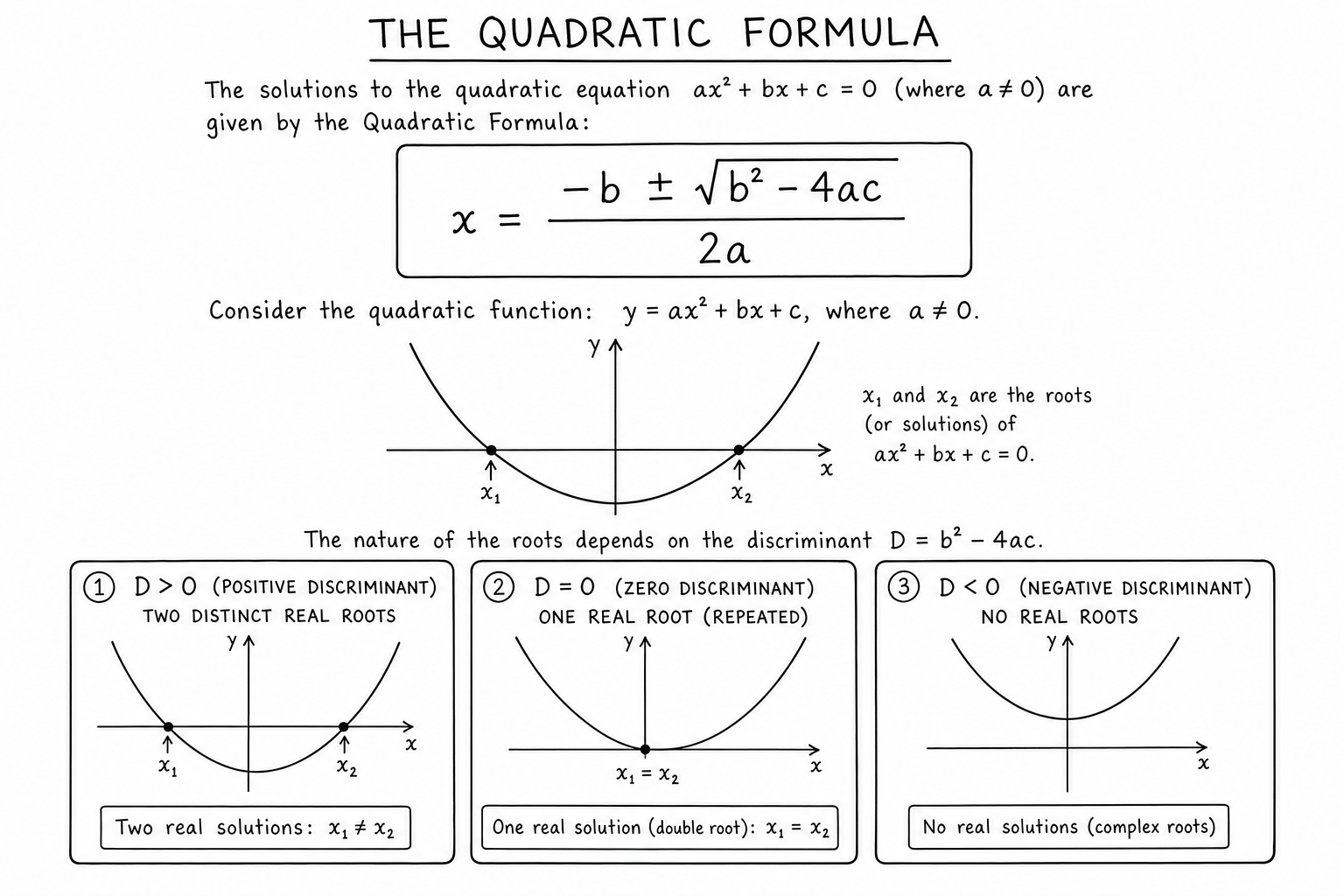
The formula is short — $x = \frac{-b \pm \sqrt{b^2 – 4ac}}{2a}$ — but encodes a complete recipe for finding roots. The expression under the square root, $b^2 – 4ac$, is the discriminant, and just by checking its sign you know how many real roots exist before computing anything else. Once you understand the discriminant, you stop solving by trial and start solving by structure.

This study note covers the formula, the derivation by completing the square, the discriminant and what it tells you, multiple worked examples, the geometric interpretation, alternative solving methods, applications across science and engineering, common pitfalls, and a brief history.

Quadratic formula equation parabola and discriminant cases modern textbook illustration

The Formula

Any equation in the standard form $ax^2 + bx + c = 0$ (with $a \neq 0$) has solutions:

$$x = \frac{-b \pm \sqrt{b^2 – 4ac}}{2a}$$

The $\pm$ sign produces two solutions in general — one taking the positive square root, one taking the negative. These are the roots of the quadratic, the values of $x$ that make the polynomial equal zero.

The formula works for any real coefficients, and even for complex coefficients with minor adjustments. It’s the unique general-purpose solver for second-degree polynomials, and it’s been the standard tool in algebra for over a thousand years.

Worked Example: Two Real Roots

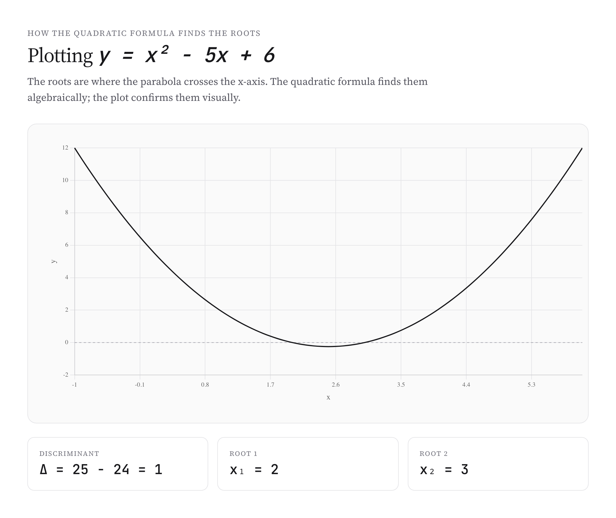
Solve $2x^2 – 4x – 6 = 0$. Here $a = 2$, $b = -4$, $c = -6$:

$$x = \frac{-(-4) \pm \sqrt{(-4)^2 – 4(2)(-6)}}{2(2)} = \frac{4 \pm \sqrt{16 + 48}}{4} = \frac{4 \pm 8}{4}$$

So $x = 3$ or $x = -1$. Two real roots, exactly what the formula promises when the discriminant is positive.

Verify by substituting back: $2(3)^2 – 4(3) – 6 = 18 – 12 – 6 = 0$ ✓; $2(-1)^2 – 4(-1) – 6 = 2 + 4 – 6 = 0$ ✓.

Worked Example: Repeated Root

Solve $x^2 – 6x + 9 = 0$. Here $a = 1$, $b = -6$, $c = 9$:

$$x = \frac{6 \pm \sqrt{36 – 36}}{2} = \frac{6 \pm 0}{2} = 3$$

One repeated root at $x = 3$. The discriminant is zero, so the $\pm$ sign doesn’t change anything. The polynomial factors as $(x – 3)^2 = 0$, which is the geometric reality behind the algebra: the parabola touches the x-axis at exactly one point, the vertex.

Worked Example: Complex Roots

Solve $x^2 + 2x + 5 = 0$. Here $a = 1$, $b = 2$, $c = 5$:

$$x = \frac{-2 \pm \sqrt{4 – 20}}{2} = \frac{-2 \pm \sqrt{-16}}{2} = \frac{-2 \pm 4i}{2} = -1 \pm 2i$$

Two complex conjugate roots: $-1 + 2i$ and $-1 – 2i$. The negative discriminant signals that the parabola never crosses the x-axis. Real-valued solutions don’t exist, but complex solutions always do — for any quadratic, the formula always gives an answer.

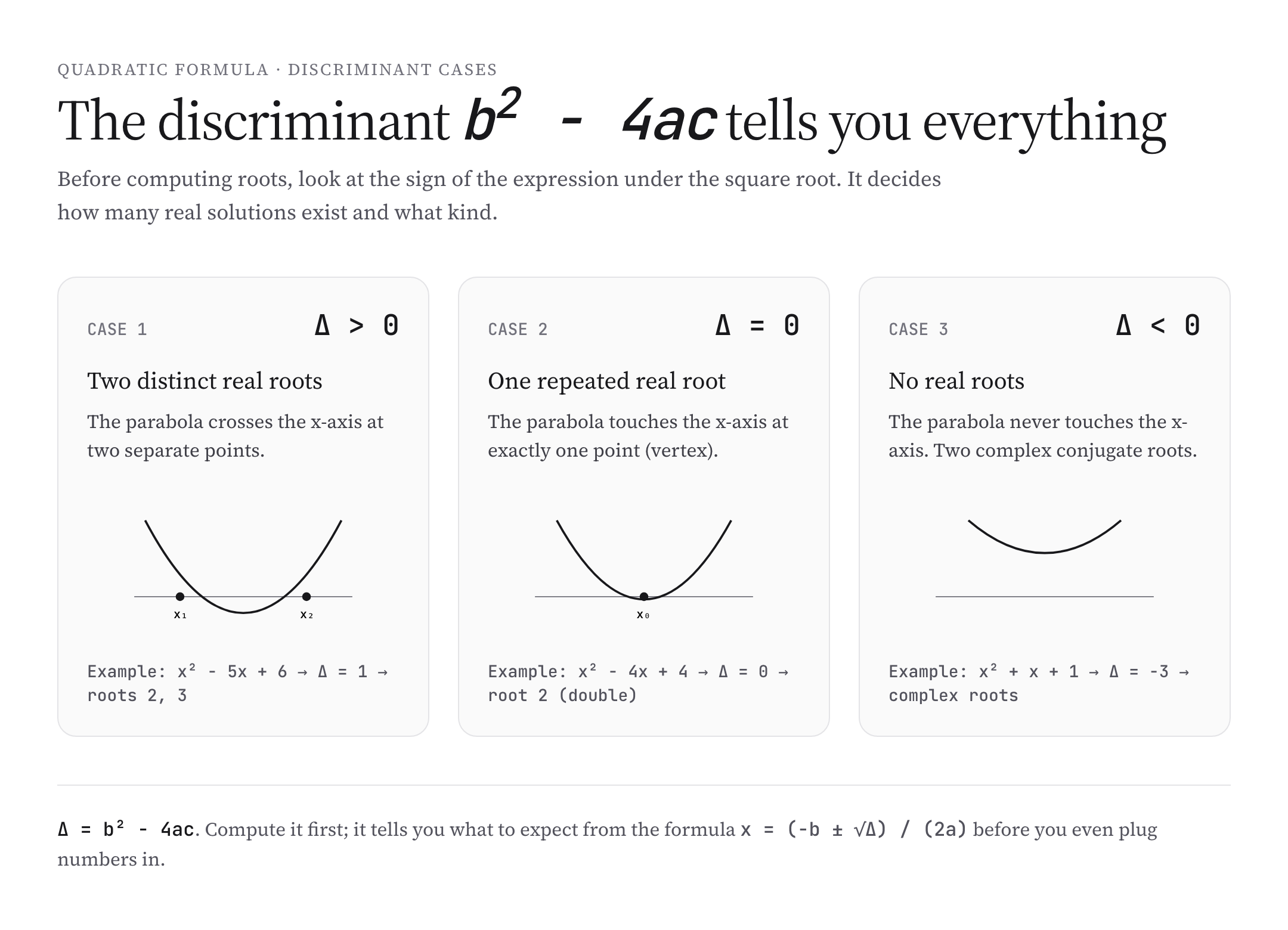
The Discriminant

The expression $\Delta = b^2 – 4ac$ under the square root is the discriminant. Its sign determines the nature of the roots:

$\Delta > 0$: two distinct real roots. The parabola crosses the x-axis at two separate points.
$\Delta = 0$: one repeated real root. The parabola touches the x-axis at exactly the vertex.
$\Delta < 0$: two complex conjugate roots. The parabola doesn’t intersect the x-axis at all.

Computing the discriminant first is the highest-leverage habit in quadratic problems. Before plugging into the formula, check the discriminant. If it’s negative and you only need real solutions, you’re done — there are none.

Discriminant cases for the quadratic formula

Derivation: Completing the Square

The quadratic formula isn’t magic; it’s the result of completing the square applied to the general quadratic. Start with $ax^2 + bx + c = 0$ and divide by $a$:

$$x^2 + \frac{b}{a} x + \frac{c}{a} = 0$$

Move the constant: $x^2 + \frac{b}{a} x = -\frac{c}{a}$. Add $(b/2a)^2$ to both sides to complete the square on the left:

$$\left(x + \frac{b}{2a}\right)^2 = \frac{b^2 – 4ac}{4a^2}$$

Take the square root of both sides:

$$x + \frac{b}{2a} = \pm \frac{\sqrt{b^2 – 4ac}}{2a}$$

Solve for $x$: $x = \frac{-b \pm \sqrt{b^2 – 4ac}}{2a}$. The formula falls out directly.

Plotting the Quadratic to Visualize Roots

The graph of $y = ax^2 + bx + c$ is a parabola. The roots of the equation are the x-coordinates where the parabola crosses the x-axis. Visualizing the curve makes the discriminant cases tangible: two crossings, one tangent point, or no crossings at all.

The vertex of the parabola sits at $x = -b/(2a)$, exactly midway between the two roots when they’re real. The y-coordinate of the vertex is $c – b^2/(4a)$. If $a > 0$ the parabola opens upward; if $a < 0$ it opens downward.

This geometric view is why quadratic optimization problems (find the maximum or minimum) are also routine — the extremum is always at the vertex, and the formula $x = -b/(2a)$ gives it directly.

Parabola y = x squared minus 5x plus 6 with roots marked

Alternative Methods: Factoring

For nice integer-coefficient quadratics, factoring is faster than the formula. To factor $x^2 + 5x + 6$, look for two numbers whose product is 6 and sum is 5: 2 and 3. So $x^2 + 5x + 6 = (x + 2)(x + 3)$, and the roots are $-2$ and $-3$.

Factoring works when integer roots exist; the formula always works. If you can’t factor in a few seconds, switch to the formula. This is the standard professional pattern: try factoring briefly for elegance, fall back on the formula for reliability.

Alternative Method: Completing the Square Manually

Completing the square (the technique we used to derive the formula) also solves quadratics directly. For $x^2 + 6x – 7 = 0$, rewrite as $(x + 3)^2 – 9 – 7 = 0$, giving $(x + 3)^2 = 16$, so $x + 3 = \pm 4$ and $x = 1$ or $x = -7$.

Completing the square is more work for routine problems but more insightful — it reveals the vertex form and the underlying algebraic structure. It’s also essential for converting any quadratic into vertex form for graphing or optimization.

Vieta’s Formulas

For $ax^2 + bx + c = 0$ with roots $r_1$ and $r_2$, Vieta’s formulas connect the roots back to the coefficients:

Sum of roots: $r_1 + r_2 = -b/a$
Product of roots: $r_1 r_2 = c/a$

These shortcuts let you verify quickly. If the roots of $x^2 – 5x + 6$ are 2 and 3, then $2 + 3 = 5 = -(-5)/1$ ✓ and $2 \times 3 = 6 = 6/1$ ✓.

Vieta’s formulas generalize to higher-degree polynomials and are widely used in algebra contests, root-finding sanity checks, and analytical work in differential equations.

Where the Quadratic Formula Shows Up

Physics: projectile motion problems involve quadratic equations because position varies as $\frac{1}{2}gt^2$. Computing landing times, ranges, and intersection points all use the quadratic formula.
Engineering: beam deflection, stress analysis, and resonant frequencies often produce quadratic equations whose roots specify critical conditions.
Optimization: finding the maximum or minimum of a quadratic objective is the textbook quadratic problem in linear and quadratic programming.
Computer graphics: ray-sphere intersection algorithms solve a quadratic in the ray parameter to find collision points.
Finance: compound interest models, internal rate of return calculations, and option pricing models all rely on quadratic (and higher-order) polynomial solving.
Statistics and machine learning: quadratic loss functions, Gaussian probability densities, and regularization terms are all quadratics whose minima have closed-form solutions via the formula.

Common Mistakes With the Quadratic Formula

Sign errors with $b$. The formula uses $-b$, so a negative $b$ becomes $+b$. Always re-read your coefficient signs after substituting.
Forgetting the $\pm$. The $\pm$ produces two solutions. Reporting only one is the most common mistake on quadratic problems.
Squaring the negative inside. $(-b)^2 = b^2$, but $-b^2 \neq b^2$. Order of operations matters: square first, then negate.
Computing the discriminant wrong. The minus sign sometimes gets dropped: $b^2 – 4ac$, not $b^2 + 4ac$.
Misidentifying $a$, $b$, $c$. Equations like $3x^2 = 5x – 2$ need to be rearranged to standard form $3x^2 – 5x + 2 = 0$ before applying the formula.
Ignoring the case $a = 0$. If $a = 0$, the equation is linear, not quadratic, and the formula produces division by zero. Check that you actually have a quadratic before applying the formula.

A Brief History of the Quadratic Formula

Babylonian mathematicians solved quadratic-like problems around 2000 BCE using completing-the-square methods, though they didn’t have algebraic notation. They worked through specific numerical examples that effectively used the formula.

Indian mathematician Brahmagupta gave a complete general solution in 628 CE, including handling negative numbers. Persian mathematician al-Khwarizmi systematically classified and solved all six standard forms of quadratic equations in the 9th century — his name gives us “algorithm” and “algebra.”

The modern algebraic notation came in the 16th and 17th centuries with François Viète and René Descartes. The compact formula $x = \frac{-b \pm \sqrt{b^2 – 4ac}}{2a}$ we use today crystallized in early modern Europe and has been a textbook staple ever since. Cubic and quartic formulas were derived in the 16th century by Cardano, Ferrari, and Tartaglia; quintic equations have no general algebraic solution, as Abel and Galois later proved.

The Quadratic in Other Forms

Beyond standard form, quadratics appear in three useful alternative forms:

Vertex form: $y = a(x – h)^2 + k$, where $(h, k)$ is the vertex. Best for graphing and optimization.
Factored form: $y = a(x – r_1)(x – r_2)$, where $r_1, r_2$ are the roots. Best when roots are known.
Standard form: $y = ax^2 + bx + c$. Best for general work and the quadratic formula.

Conversion between forms is routine algebra. Completing the square turns standard form into vertex form. Factoring (or applying the formula) turns standard form into factored form. Expanding turns vertex or factored form back into standard form. Knowing all three forms and switching between them efficiently is the practical fluency that separates routine algebra from real problem-solving.

Quadratic Inequalities

The quadratic formula also handles inequalities like $ax^2 + bx + c > 0$ or $< 0$. Find the roots, then check which intervals satisfy the inequality.

For $x^2 – 4x + 3 > 0$, the roots are 1 and 3. The parabola opens upward, so it’s negative between the roots and positive outside them. The inequality holds for $x < 1$ or $x > 3$.

Quadratic inequalities show up in optimization problems with constraints, regions in the plane defined by polynomial bounds, and stability analysis where a quadratic discriminant must remain positive (or negative) for a system to remain stable.

Quadratic Optimization

Many real problems reduce to “minimize or maximize a quadratic.” The vertex of $y = ax^2 + bx + c$ sits at $x = -b/(2a)$, and substituting back gives the optimal value. If $a > 0$, the vertex is a minimum; if $a < 0$, it's a maximum.

Linear regression’s least-squares solution falls out of minimizing a sum of squared residuals — a quadratic in the coefficients. Optimal control problems with quadratic cost functions (LQR controllers in engineering) have closed-form solutions because the Hessian is constant. Anywhere the cost is naturally quadratic, the formula gives the optimum without iteration.

Numerical Stability of the Quadratic Formula

The standard formula has a hidden numerical trap. When $b^2 \gg |4ac|$, the expression $-b + \sqrt{b^2 – 4ac}$ suffers catastrophic cancellation — two nearly-equal large numbers subtract to a tiny one, losing precision.

The fix: compute one root with the formula, then use Vieta’s product $r_1 r_2 = c/a$ to derive the second. $r_2 = c / (a \cdot r_1)$ avoids the cancellation problem entirely. Production numerical libraries (LAPACK, GSL, NumPy) implement this stabilized version, not the textbook formula. The standard formula is correct mathematically and dangerous numerically — a useful reminder that “exact algebra” and “stable computation” aren’t always the same thing.

Reducing Higher-Degree Polynomials to Quadratics

Some polynomials of degree 4 or higher reduce to quadratics through substitution. $x^4 – 5x^2 + 6 = 0$ becomes a quadratic in $u = x^2$: $u^2 – 5u + 6 = 0$. Solving gives $u = 2$ or $u = 3$, so $x^2 = 2$ or $x^2 = 3$, and the four roots are $\pm\sqrt{2}, \pm\sqrt{3}$.

This biquadratic trick works whenever a polynomial has only even powers (or only powers in arithmetic progression). It reduces what looks like a hard problem to two routine quadratic solves. Many physics problems involving energy minimization, optical path lengths, and resonance frequencies produce biquadratics; the substitution turns them into instantly solvable problems.

Quadratic Forms in Higher Dimensions

A quadratic form in two variables is $Q(x, y) = ax^2 + bxy + cy^2$. The discriminant $b^2 – 4ac$ classifies conic sections: positive gives a hyperbola, zero gives a parabola, negative gives an ellipse.

Quadratic forms generalize to any number of variables. They’re the multivariable analogue of single-variable quadratics, written compactly as $Q(\mathbf{x}) = \mathbf{x}^T A \mathbf{x}$ for a symmetric matrix $A$. Eigenvalues of $A$ classify the form: all positive means the quadratic form is positive definite (used heavily in optimization). Mixed eigenvalue signs give saddle points.

Quadratic Formula in Programming

Implementing the quadratic formula in code looks trivial but has subtle pitfalls. Here’s a robust Python implementation:

import math
def solve_quadratic(a, b, c):
    if a == 0:
        if b == 0: return [] if c != 0 else 'all reals'
        return [-c / b]
    disc = b*b - 4*a*c
    if disc < 0:
        re = -b / (2*a)
        im = math.sqrt(-disc) / (2*a)
        return [complex(re, im), complex(re, -im)]
    if disc == 0:
        return [-b / (2*a)]
    # Use Vieta's formula for numerical stability
    sqrt_d = math.sqrt(disc)
    if b > 0:
        r1 = (-b - sqrt_d) / (2*a)
    else:
        r1 = (-b + sqrt_d) / (2*a)
    r2 = c / (a * r1)
    return [r1, r2]

Notice the explicit handling of degenerate cases (a = 0, repeated roots, complex roots) and the numerically stable computation that avoids catastrophic cancellation. Production scientific libraries (NumPy, SciPy, GSL) follow the same patterns.

FAQs

Why does the quadratic formula always work?

Because it’s derived from the universal technique of completing the square, which works on any quadratic equation. The formula encodes the full recipe in one expression, including the discriminant case structure for real, repeated, or complex roots.

What does the discriminant tell me?

The discriminant b² − 4ac determines the nature of the roots. Positive: two distinct real roots. Zero: one repeated real root. Negative: two complex conjugate roots. Computing it first tells you what to expect before doing the full formula evaluation.

When should I factor instead of using the formula?

When the quadratic has obvious integer roots, factoring is faster. Look for two numbers that multiply to c (or c/a) and add to b (or b/a). If you can’t factor in 30 seconds, switch to the formula — it always works, even when factoring fails.

Why is there a ± sign in the formula?

Because the square root produces both a positive and a negative value. The two values give two solutions, which are the two intersections of the parabola with the x-axis. Quadratics have exactly two roots (counted with multiplicity, over the complex numbers).

Can the quadratic formula give complex solutions?

Yes — when the discriminant is negative, the square root produces an imaginary number, and the roots become complex conjugates of the form a ± bi. Complex roots are mathematically valid; they just don’t correspond to x-axis intersections in real space.

How do I know which form to use: standard, vertex, or factored?

Standard form is best for the formula and general manipulation. Vertex form is best for graphing and finding extrema. Factored form is best when roots are known. Practice converting between all three and switching based on what the problem needs.

What is completing the square?

An algebraic technique that rewrites a quadratic ax² + bx + c as a(x − h)² + k. It’s the derivation engine behind the quadratic formula and the standard way to convert standard form into vertex form. Worth practicing because it generalizes to many other algebra problems.

Who discovered the quadratic formula?

Pieces of it date back to Babylonian mathematicians (~2000 BCE). Brahmagupta gave a complete general solution in 628 CE. Al-Khwarizmi systematized quadratic solving in the 9th century. The modern notation crystallized in the 16th and 17th centuries with Viète and Descartes.

What is Vieta’s formula for quadratics?

For roots r₁ and r₂ of ax² + bx + c = 0: sum r₁ + r₂ = −b/a, product r₁r₂ = c/a. These let you verify your solutions and sometimes find roots faster than the formula by inspection.

How is the quadratic formula used in physics?

Projectile motion is the most common application. Position varies as ½gt², which gives a quadratic in time. Solving for landing time, time of flight, or intersection times all use the quadratic formula. Other uses include resonant frequency calculations and beam deflection analysis.

What happens when a = 0 in the formula?

The equation becomes linear (bx + c = 0), not quadratic. The formula’s denominator is 2a, which would be zero — the formula doesn’t apply. Check that a ≠ 0 before using the quadratic formula. For linear equations, just solve x = −c/b directly.

Can quadratic equations have more than two roots?

No. The fundamental theorem of algebra says a degree-n polynomial has exactly n roots over the complex numbers, counted with multiplicity. A quadratic has exactly two roots, which may be distinct real, equal real, or complex conjugates.

Why does the quadratic formula sometimes give numerically wrong answers in software?

Because of catastrophic cancellation when |b| is much larger than √(b²−4ac). Subtracting two nearly equal large numbers loses precision. Stable implementations compute one root with the formula and the other from Vieta’s product r₁r₂ = c/a.