The Normal Distribution

Q: Why is the normal distribution so important in statistics?

Because of the central limit theorem: averages of large samples tend toward normal regardless of the underlying distribution. This makes the normal distribution the natural model for sample means, regression residuals, and most classical inference.

Q: What's the difference between a normal distribution and a standard normal distribution?

A standard normal has mean 0 and standard deviation 1. Any normal distribution can be converted to a standard normal by computing z-scores. Standardizing makes lookup tables and software functions universally usable.

Q: How do I know if my data is normally distributed?

Plot a histogram and a Q-Q plot first — eye it. Then run a Shapiro-Wilk test (small samples) or Anderson-Darling test (larger samples). Real data is rarely perfectly normal; the question is whether the deviation matters for your analysis.

Q: What is the 68-95-99.7 rule?

It's the empirical rule for normal distributions: 68% of values fall within ±1 standard deviation of the mean, 95% within ±2σ, and 99.7% within ±3σ. Useful for quick mental estimates of where most data sits.

Q: When should I not assume a normal distribution?

When data is skewed, when extreme outliers are common, when the variable is bounded (probabilities between 0 and 1, counts that can't go negative), or when sample size is small and you don't have a clear theoretical reason for normality. Use t-distributions, log-normal, beta, or non-parametric methods instead.

Q: Who discovered the normal distribution?

Abraham de Moivre first described it in 1733 as the limit of binomial distributions. Carl Friedrich Gauss popularized it in 1809 in his work on astronomical observations, which is why it's also called the Gaussian distribution. Pierre-Simon Laplace did parallel work on the error distribution.

Q: What's the relationship between normal and binomial distributions?

For large n with success probability p not too close to 0 or 1, the binomial distribution is approximately normal with mean np and variance np(1−p). This is the de Moivre-Laplace theorem and is the historical origin of the normal distribution.

Q: How is the normal distribution used in machine learning?

Linear regression assumes normal errors. Gaussian discriminant analysis models class-conditional densities as multivariate normal. Gaussian processes use it for non-parametric regression. Variational autoencoders use Gaussian latent variables. Even neural network weight initialization typically samples from a normal distribution.

Q: What is a multivariate normal distribution?

It's the generalization to multiple correlated variables. Parameterized by a mean vector and a covariance matrix, it's the foundation for principal component analysis, Gaussian mixture models, Kalman filters, and many other multivariate techniques.

Q: Why does the normal distribution have a strange formula?

The 1/(σ√(2π)) factor is the normalizing constant that makes the total area equal to 1. The exponential of −(x−μ)²/2σ² creates the symmetric bell shape with peak at μ and inflection points at ±σ. The formula's complexity comes from the math of probability density functions, not from the underlying intuition, which is actually quite simple — values cluster around the mean and become exponentially rarer as you move away.

The normal distribution is the symmetric bell-shaped curve at the center of classical statistics. Heights, measurement errors, IQ scores, average sums of independent variables — they all tend toward this shape. Most statistical tests assume it. Most confidence intervals are built from it. Most machine learning algorithms have a normal-distribution assumption hiding somewhere in their derivation.

Knowing the normal distribution well does two things. It lets you read any chart marked in standard deviations on sight. And it makes you suspicious of the model when reality has fat tails — the normal distribution underweights extreme events, which is why crashes and outliers keep surprising people who only carry it in their head.

This study note covers the formula, parameters, properties, the standard normal, z-scores, the central limit theorem connection, the empirical rule, history, applications across science and finance, and the situations where the normal distribution is the wrong model and you need something else.

Normal distribution bell curve formula and properties modern textbook illustration

The Formula

A normal distribution with mean $\mu$ and standard deviation $\sigma$ has probability density:

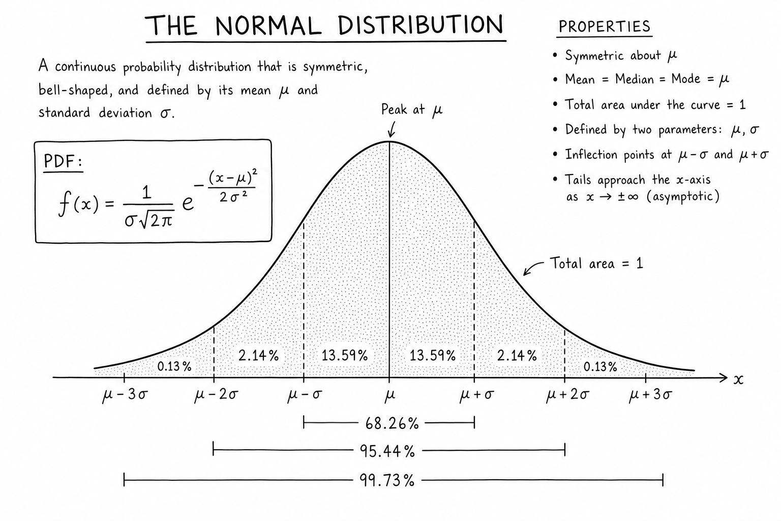
$$f(x) = \frac{1}{\sigma\sqrt{2\pi}} \, e^{-\frac{(x-\mu)^2}{2\sigma^2}}$$

Two parameters fully describe it. $\mu$ sets where the peak sits. $\sigma$ sets how wide the bell is. The total area under the curve always equals 1 (it’s a probability density).

Notation: $X \sim N(\mu, \sigma^2)$ means $X$ is normally distributed with mean $\mu$ and variance $\sigma^2$. Some textbooks write the second parameter as $\sigma$ instead of $\sigma^2$; always check which convention the source uses.

Properties That Make Normal Special

Symmetric around the mean. Skewness is zero.
Mean = median = mode. All three measures of central tendency coincide at $\mu$.
Inflection points at $\mu \pm \sigma$ — where the curve transitions from concave-down to concave-up.
Tails approach the x-axis asymptotically but never touch it; technically, normal distributions have unbounded support.
Linear combinations of normals are normal. If $X \sim N(\mu_1, \sigma_1^2)$ and $Y \sim N(\mu_2, \sigma_2^2)$ are independent, then $aX + bY \sim N(a\mu_1 + b\mu_2, a^2\sigma_1^2 + b^2\sigma_2^2)$. This closure property is rare and powerful — it lets entire fields of statistics build cleanly on normal assumptions.
Maximum entropy for a given mean and variance among continuous distributions on the real line. In an information-theoretic sense, the normal is the “least committed” choice.

The Standard Normal Distribution

The standard normal distribution is the special case with $\mu = 0$ and $\sigma = 1$. It’s denoted $Z \sim N(0,1)$ and is the reference for z-tables.

$$\phi(z) = \frac{1}{\sqrt{2\pi}} e^{-z^2/2}$$

Any normal random variable can be transformed to a standard normal by subtracting the mean and dividing by the standard deviation. That transformation is the z-score (next section).

Z-Scores: Standardizing Any Normal

To compare a value across normal distributions with different means and spreads, convert to a z-score:

$$z = \frac{x – \mu}{\sigma}$$

A z-score is the number of standard deviations a value sits above or below the mean. $z = 1.5$ means the value is 1.5σ above the mean, regardless of the original units. Z-scores let you look up tail probabilities in a standard normal table.

For a normally distributed test where $\mu = 70$ and $\sigma = 10$, a score of 85 corresponds to $z = 1.5$. Standard tables show $P(Z < 1.5) \approx 0.933$, so 85 sits at roughly the 93rd percentile.

Z-scores show up everywhere in applied statistics — outlier flagging (often $|z| > 3$), portfolio risk reports, A/B test analysis, and quality control charts. They also generalize to multivariate normal data via Mahalanobis distance, which accounts for correlations between variables.

The 68-95-99.7 Rule

For any normal distribution, predictable shares of the data sit within standard-deviation bands around the mean:

About 68% of values fall within ±1σ.
About 95% fall within ±2σ (more precisely, ±1.96σ for exactly 95%).
About 99.7% fall within ±3σ.

Memorize these three numbers. They turn any “the mean is 100, σ is 15” report into an instant range estimate (about 70–130 covers most cases). They’re also the source of the “two-sigma” and “three-sigma” thresholds in quality control and finance.

Central Limit Theorem Connection

The normal distribution dominates because of the central limit theorem: when you sum many independent random variables, the result tends toward normal even if the inputs aren’t. Heights are a sum of many genetic and environmental factors. Measurement errors are sums of many small random influences. Sample means are averages of many observations.

This is also why the normal distribution shows up so often in business statistics, data science, and machine learning even when the underlying data isn’t itself normal.

A Brief History

The normal distribution was first described by Abraham de Moivre in 1733 as a limit of the binomial distribution. Pierre-Simon Laplace generalized it in his work on errors. Carl Friedrich Gauss popularized it in 1809 in his analysis of astronomical observations, which is why it’s also called the Gaussian distribution. Adolphe Quetelet in the 1830s applied it to human characteristics, founding “social physics” and the idea of the average man.

The 20th century cemented its central role. Sir Francis Galton introduced the idea of regression to the mean using normal-distribution thinking. R.A. Fisher, Jerzy Neyman, and Egon Pearson built classical inference on normal-based test statistics. Modern statistics still defaults to normal assumptions in most introductory and applied work.

Applications Across Disciplines

Education and psychology. Standardized test scores (SAT, ACT, GRE, IQ) are designed to be normally distributed by construction.
Quality control. Process control charts use normal distribution assumptions to set ±3σ limits and detect out-of-control behavior.
Finance. Black-Scholes option pricing assumes log-normal stock prices (so log returns are normal). Value at Risk calculations often assume normal returns. The crashes that follow when reality disagrees are a recurring lesson.
Engineering. Tolerance stack-up analysis assumes normal distributions of component dimensions. Reliability engineering uses normal assumptions for stress-strength models.
Biology. Many biological measurements (height, blood pressure, enzyme activity) are approximately normal because they’re sums of many small genetic and environmental contributions.
Machine learning. Linear regression, Gaussian discriminant analysis, Gaussian processes, variational autoencoders — all built on normal-distribution foundations.

Where the Model Breaks

The normal distribution underestimates extreme events. Real-world phenomena with fat tails — stock returns, network traffic, earthquake magnitudes, viral spread — produce far more 4σ and 5σ events than the formula predicts. The 2008 crisis was repeatedly described as a “25-sigma event” by analysts using normal-distribution risk models, which is to say their models were wrong, not that the universe glitched.

For phenomena where extremes matter, switch to t-distributions, log-normal distributions, or Pareto/power-law models. The normal distribution is the right starting point and the wrong stopping point for risk-sensitive work.

Other failure modes:

Bounded data. Probabilities are between 0 and 1. Counts can’t go negative. Use beta, binomial, or Poisson distributions instead.
Skewed data. Income, time-to-failure, and many natural processes are right-skewed. Log-normal or gamma distributions usually fit better.
Multimodal data. Mixtures of populations (e.g., heights in a mixed-gender sample) produce two peaks. Mixture models, not single normals, are appropriate.
Small samples from non-normal distributions. The central limit theorem is asymptotic. With small $n$, the sample mean of a heavy-tailed distribution is still heavy-tailed.

Multivariate Normal Distribution

The multivariate normal generalizes the bell curve to multiple correlated variables. Parameters: a mean vector $\boldsymbol{\mu}$ and a covariance matrix $\boldsymbol{\Sigma}$. The density is:

$$f(\mathbf{x}) = \frac{1}{(2\pi)^{k/2} |\boldsymbol{\Sigma}|^{1/2}} \exp\left(-\frac{1}{2}(\mathbf{x} – \boldsymbol{\mu})^T \boldsymbol{\Sigma}^{-1} (\mathbf{x} – \boldsymbol{\mu})\right)$$

The covariance matrix encodes both individual variances (diagonal entries) and pairwise correlations (off-diagonal entries). Multivariate normal is the foundation for principal component analysis, Gaussian mixture models, Kalman filters, and Gaussian processes.

The Lognormal Distribution and Why Skewed Data Often Looks This Way

If $X$ is normally distributed, then $e^X$ is lognormally distributed — heavily right-skewed with a long tail. Many real-world variables that are products of many small independent factors (incomes, stock prices, particle sizes, file sizes) are approximately lognormal because the log of a product of independents is a sum, and sums tend toward normal by the CLT.

For analysis of lognormal data, taking the logarithm first often restores normal-distribution assumptions and lets you use standard parametric methods. Log returns in finance, log-transformed expression values in genomics, and log-scaled web traffic counts are everyday examples.

Q-Q Plots and Normality Testing

The quickest visual check for normality is a quantile-quantile (Q-Q) plot: plot sample quantiles against theoretical normal quantiles. A straight diagonal line means the data is approximately normal. Curvature at the ends signals heavy tails. S-shapes indicate skewness.

Formal tests include:

Shapiro-Wilk: best for small to moderate samples (n < 5000). Sensitive to all forms of non-normality.
Anderson-Darling: good general-purpose test, especially for tail behavior.
Kolmogorov-Smirnov: compares cumulative distributions; less powerful than Shapiro-Wilk against alternatives that share the same mean and variance.

For large samples, even tiny deviations from normality become statistically significant. Visual inspection often matters more than test results — the question is whether the deviation matters for your downstream analysis, not whether it’s detectable.

Confidence Intervals from the Normal Distribution

For a sample mean $\bar{x}$ with known standard error $SE$, the 95% confidence interval is approximately:

$$\bar{x} \pm 1.96 \times SE$$

The 1.96 comes from the standard normal distribution: $P(|Z| < 1.96) = 0.95$. For 99% confidence, use 2.576. For 90%, use 1.645.

When standard deviation is unknown and estimated from the sample (the usual case), use the t-distribution instead, which has slightly wider tails. For large samples, t and normal are nearly identical and the 1.96 multiplier still works well.

This formula is the backbone of polling margins of error, scientific paper confidence intervals, and most “estimate ± uncertainty” reports in applied work.

The Normal Distribution in Hypothesis Testing

One-sample z-tests compare a sample mean to a hypothesized population mean using the test statistic:

$$z = \frac{\bar{x} – \mu_0}{\sigma / \sqrt{n}}$$

If $|z|$ exceeds a critical value (1.96 for two-sided test at $\alpha = 0.05$), reject the null hypothesis. The p-value is twice the probability that $Z$ exceeds $|z|$ under the standard normal.

Two-sample z-tests compare two means; they use a similar test statistic with pooled standard error. Most modern A/B test calculators automate this, but the underlying math is simple normal-distribution mechanics.

Why Many Real Variables Are Approximately Normal

Three reinforcing reasons:

Central limit theorem. Sums of many independent random variables tend toward normal. Many real-world quantities (heights, errors, biological traits, sample averages) arise as such sums.
Maximum entropy. Among continuous distributions on the real line with given mean and variance, the normal has the most entropy. In an information-theoretic sense, it’s the most “non-committal” choice when only the mean and variance are known.
Mathematical convenience. Normal distributions are closed under linear combinations, easy to integrate, and have well-understood properties. Statistical theory grew around the normal because the math worked out cleanly.

Common Misconceptions About the Normal Distribution

“Most data is normally distributed.” No — most real data is skewed, bounded, or otherwise non-normal. Sample means tend to normal; raw data often doesn’t.
“Outliers are impossible if the data is normal.” Outliers happen — about 0.3% of values exceed ±3σ for an exactly normal distribution. For real data with fatter tails, true outliers are even more common.
“Z-scores work for any distribution.” Z-score formulas can be applied to any distribution, but the percentile interpretation only holds for normals. A z-score of 2 corresponds to the 97.5th percentile only if the data is normal.
“Bigger samples mean more normality.” The sampling distribution of the mean becomes more normal with larger samples. The underlying data does not become more normal — it stays whatever shape it always was.

Why the Normal Distribution Is Sometimes Called Gaussian

The terms “normal distribution” and “Gaussian distribution” refer to the same object. Gauss popularized it in 1809 in his work on the method of least squares applied to astronomical observations, which is why it bears his name. The term “normal” was coined later by Karl Pearson, who pushed back when reviewers complained the name implied other distributions were “abnormal.” Pearson stuck with it; the name stuck with the discipline.

Most modern textbooks use the two terms interchangeably. Statisticians often prefer “normal” as the default term in inference contexts; physicists and engineers often prefer “Gaussian” because it ties cleanly to Gaussian processes, Gaussian integrals, and Gaussian wave packets across applied math.

Worked Example: SAT Scores

SAT section scores are designed to follow a normal distribution with mean approximately 500 and standard deviation approximately 100 (per section, on the older 200–800 scale). A student scores 650. What percentile is that?

Z-score: $z = (650 – 500) / 100 = 1.5$. Standard normal table gives $P(Z < 1.5) \approx 0.933$. The student is at the 93rd percentile — better than 93% of test takers.

This kind of percentile mapping is the entire reason standardized tests use normal-distribution score scales. Test designers calibrate raw scores into a normal distribution so that scaled scores map cleanly to percentiles, regardless of how the raw question difficulty turned out that year.

Skewness and Kurtosis: When Normal Doesn’t Fit

Two diagnostic statistics tell you whether a distribution looks normal:

Skewness measures asymmetry. Zero for symmetric distributions; positive for right-skewed (long tail to the right); negative for left-skewed.
Kurtosis measures tail heaviness. Three for normal; greater than three for fat-tailed (more extreme events than normal predicts); less than three for light-tailed.

Many practitioners report excess kurtosis (kurtosis − 3) so that a normal distribution has zero excess kurtosis. Stock returns typically show excess kurtosis above 3 — far more 4σ and 5σ events than normal models predict. This is the formal way to quantify “fat tails” and decide whether normal assumptions are safe.

FAQs

Why is the normal distribution so important in statistics?

Because of the central limit theorem: averages of large samples tend toward normal regardless of the underlying distribution. This makes the normal distribution the natural model for sample means, regression residuals, and most classical inference.

What’s the difference between a normal distribution and a standard normal distribution?

A standard normal has mean 0 and standard deviation 1. Any normal distribution can be converted to a standard normal by computing z-scores. Standardizing makes lookup tables and software functions universally usable.

How do I know if my data is normally distributed?

Plot a histogram and a Q-Q plot first — eye it. Then run a Shapiro-Wilk test (small samples) or Anderson-Darling test (larger samples). Real data is rarely perfectly normal; the question is whether the deviation matters for your analysis.

What is the 68-95-99.7 rule?

It’s the empirical rule for normal distributions: 68% of values fall within ±1 standard deviation of the mean, 95% within ±2σ, and 99.7% within ±3σ. Useful for quick mental estimates of where most data sits.

When should I not assume a normal distribution?

When data is skewed, when extreme outliers are common, when the variable is bounded (probabilities between 0 and 1, counts that can’t go negative), or when sample size is small and you don’t have a clear theoretical reason for normality. Use t-distributions, log-normal, beta, or non-parametric methods instead.

Who discovered the normal distribution?

Abraham de Moivre first described it in 1733 as the limit of binomial distributions. Carl Friedrich Gauss popularized it in 1809 in his work on astronomical observations, which is why it’s also called the Gaussian distribution. Pierre-Simon Laplace did parallel work on the error distribution.

What’s the relationship between normal and binomial distributions?

For large n with success probability p not too close to 0 or 1, the binomial distribution is approximately normal with mean np and variance np(1−p). This is the de Moivre-Laplace theorem and is the historical origin of the normal distribution.

How is the normal distribution used in machine learning?

Linear regression assumes normal errors. Gaussian discriminant analysis models class-conditional densities as multivariate normal. Gaussian processes use it for non-parametric regression. Variational autoencoders use Gaussian latent variables. Even neural network weight initialization typically samples from a normal distribution.

What is a multivariate normal distribution?

It’s the generalization to multiple correlated variables. Parameterized by a mean vector and a covariance matrix, it’s the foundation for principal component analysis, Gaussian mixture models, Kalman filters, and many other multivariate techniques.

Why does the normal distribution have a strange formula?

The 1/(σ√(2π)) factor is the normalizing constant that makes the total area equal to 1. The exponential of −(x−μ)²/2σ² creates the symmetric bell shape with peak at μ and inflection points at ±σ. The formula’s complexity comes from the math of probability density functions, not from the underlying intuition, which is actually quite simple — values cluster around the mean and become exponentially rarer as you move away.

What’s the difference between probability density and probability for a normal distribution?

Probability density f(x) at a point isn’t a probability — it’s a rate. Probabilities come from integrating density over an interval: P(a < X < b) = ∫ₐᵇ f(x) dx. The probability of any single exact value is zero for continuous distributions, including normal.

How is the normal distribution used in finance and risk management?

Volatility (annualized standard deviation of log returns) is the headline risk metric. Value at Risk uses normal-distribution quantiles for downside estimates. Black-Scholes option pricing assumes log-normal stock prices. The 2008 crisis and similar events highlight the limits — real markets have fatter tails than normal models predict.

Why do we use 1.96 for 95% confidence intervals?

Because P(|Z| < 1.96) = 0.95 for a standard normal distribution. So a confidence interval of ±1.96 standard errors around an estimate has 95% probability of containing the true parameter (under repeated sampling). 1.96 is often rounded to 2 in informal usage, but 1.96 is the precise value.