Heisenberg Uncertainty Principle

The Heisenberg uncertainty principle says that certain pairs of physical properties — most famously position and momentum — cannot both be measured arbitrarily precisely. The more precisely you know one, the less precisely you can know the other. The bound is fundamental: it’s not a limitation of measurement technology but a property of nature itself, baked into the structure of quantum mechanics.

Werner Heisenberg formulated it in 1927, and it stands as one of the most famous and most misunderstood ideas in physics. Popular culture treats it as a vague metaphor for “you can’t know everything,” but the actual statement is precise: \(\Delta x \cdot \Delta p \geq \hbar / 2\), and similar inequalities apply to other pairs of “complementary” observables. The principle reshapes everything from atomic stability to electron microscope design to the lower bound on energy in quantum systems.

This study note covers the position-momentum statement, the energy-time relation, the underlying mathematics, common misconceptions, applications across physics and engineering, the limits of the principle, and the historical context that explains why Heisenberg’s discovery defined the philosophical character of quantum mechanics.

The Position-Momentum Statement

For any quantum particle:

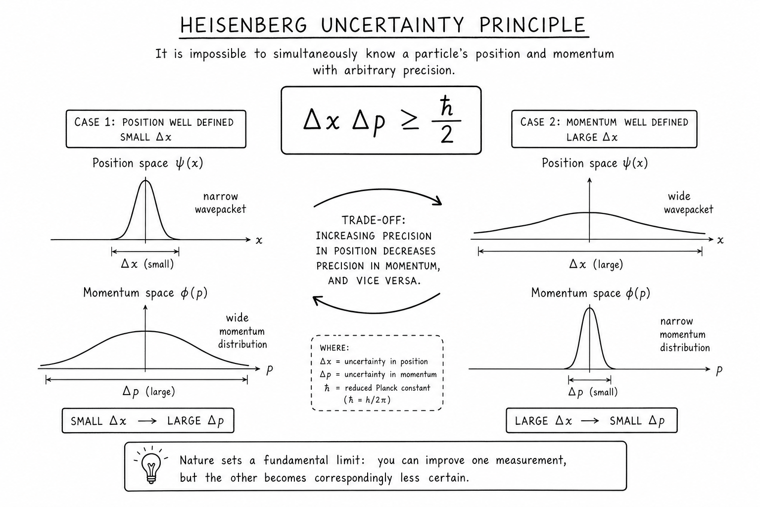
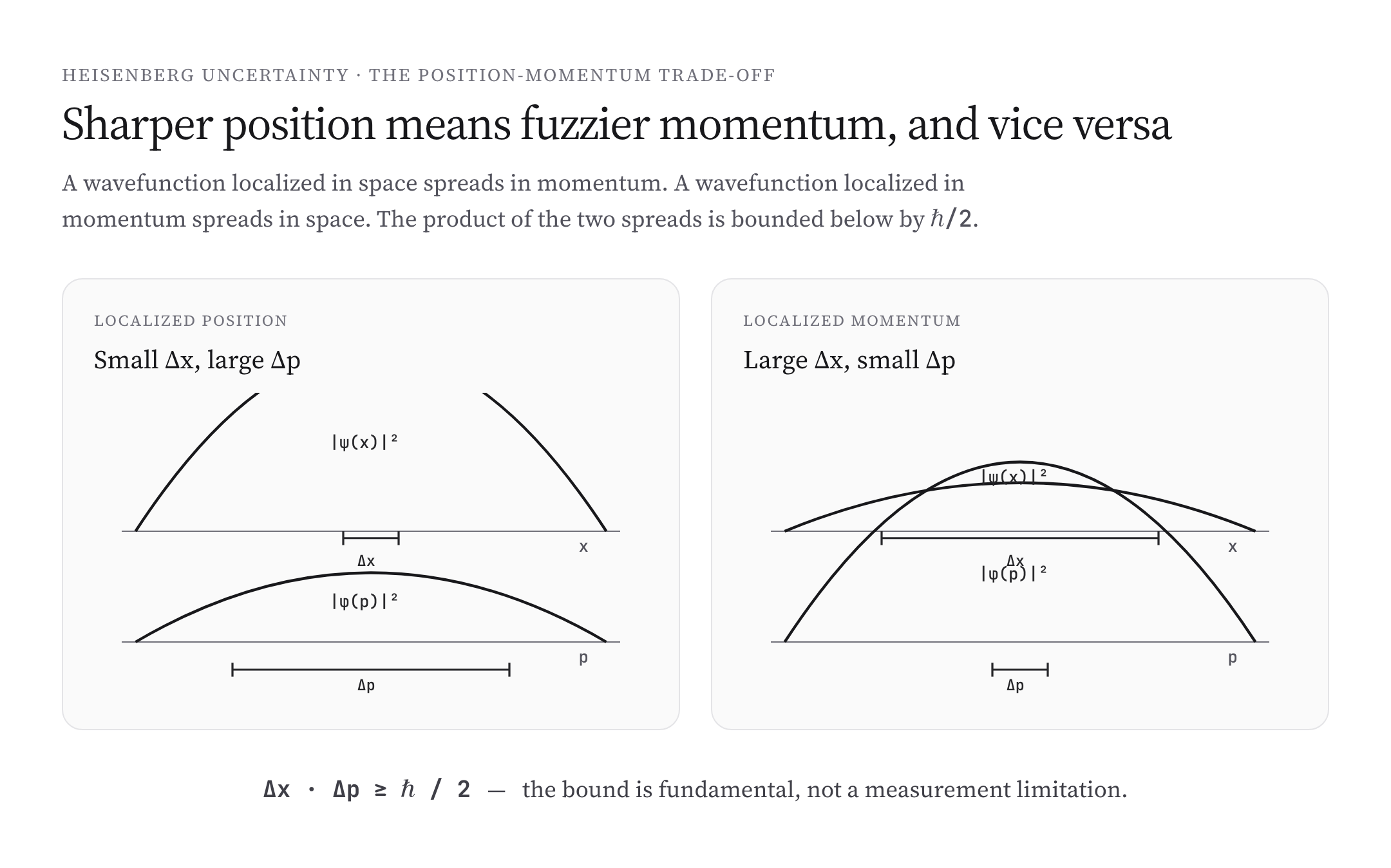
$$\Delta x \cdot \Delta p \geq \frac{\hbar}{2}$$

where \(\Delta x\) is the standard deviation of position and \(\Delta p\) is the standard deviation of momentum. Both \(\Delta x\) and \(\Delta p\) refer to spreads in the underlying probability distributions for position and momentum, not measurement errors. Even with perfect instruments, the product of these spreads cannot fall below \(\hbar/2\).

The reduced Planck constant \(\hbar = h/(2\pi) \approx 1.055 \times 10^{-34}\) J·s sets the scale. For everyday objects, \(\hbar/2\) is so tiny that the uncertainty product is utterly unmeasurable. For atoms and subatomic particles, the uncertainty bound is comparable to typical position and momentum scales, and it shapes their behavior fundamentally.

Why Position and Momentum Cannot Both Be Sharp

The reason is mathematical: in quantum mechanics, the position-space wavefunction \(\psi(x)\) and the momentum-space wavefunction \(\phi(p)\) are Fourier transforms of each other. A function localized sharply in position spreads broadly in frequency (and hence momentum); a function with a narrow frequency content extends over a wide range in space. The Fourier transform forces a trade-off — making one narrow makes the other wide.

This trade-off shows up in classical wave physics too: a brief sound pulse contains a wide range of frequencies; a pure tone (single frequency) requires an infinite duration. Heisenberg’s principle is the quantum mechanical version, where position and momentum are conjugate variables related by the Fourier transform.

Worked Example: An Electron in an Atom

An electron is confined to roughly the size of a hydrogen atom: \(\Delta x \sim 10^{-10}\) m. The minimum momentum uncertainty is:

$$\Delta p \geq \hbar / (2 \Delta x) \approx 5 \times 10^{-25} \text{ kg m/s}$$

The corresponding kinetic energy uncertainty: \(\Delta E \sim p^2/(2m_e) \sim 1.4 \times 10^{-19}\) J ≈ 0.9 eV. The actual ground state energy of hydrogen is 13.6 eV — same order of magnitude. This isn’t coincidence: the size of atoms and their characteristic energies are set by Heisenberg’s principle. An electron confined to a smaller volume would have higher kinetic energy; the balance between kinetic energy and Coulomb attraction determines atomic size.

This is also why atoms are stable. Classical mechanics predicts that an electron orbiting a nucleus should radiate energy and spiral in. Heisenberg’s principle prevents this — squeezing the electron’s position too much raises its momentum (and kinetic energy) to the point where it can no longer be bound. Atoms exist with their actual sizes precisely because of the uncertainty principle.

Other Conjugate Pairs

The position-momentum relation generalizes to any pair of “complementary” or “conjugate” observables. The general statement: for two observables \(A\) and \(B\) with operators \(\hat{A}\) and \(\hat{B}\):

$$\Delta A \cdot \Delta B \geq \frac{1}{2} |\langle [\hat{A}, \hat{B}] \rangle|$$

where \([\hat{A}, \hat{B}] = \hat{A}\hat{B} – \hat{B}\hat{A}\) is the commutator. For position and momentum, \([\hat{x}, \hat{p}] = i\hbar\), giving the standard \(\Delta x \cdot \Delta p \geq \hbar/2\).

Other pairs include orthogonal components of angular momentum (e.g., \(L_x\) and \(L_y\)), components of spin (\(S_x\) and \(S_z\)), and certain field-conjugate momentum pairs in quantum field theory.

The Energy-Time Uncertainty Relation

A separate but related uncertainty inequality involves energy and time:

$$\Delta E \cdot \Delta t \geq \frac{\hbar}{2}$$

The interpretation differs from the position-momentum case. Time isn’t an operator in standard quantum mechanics, so \(\Delta t\) doesn’t have the same direct meaning as \(\Delta x\). Several common interpretations:

• \(\Delta t\) is the lifetime of a quantum state; \(\Delta E\) is the natural width of its energy.
• \(\Delta t\) is the time required to measure energy with precision \(\Delta E\).
• \(\Delta E\) is the energy fluctuation possible during a process of duration \(\Delta t\), as in virtual particles in quantum field theory.

This relation explains why excited atomic states have natural linewidths in their emission spectra (short-lived states have larger linewidths) and why virtual particles in quantum field theory can briefly violate energy conservation.

Common Misconceptions

1. “It’s about measurement disturbing the system.” Partly true but not fundamental. Even if no measurement occurs, the uncertainty bound holds for the underlying probability distributions of position and momentum. The principle reflects the structure of quantum mechanics, not just measurement physics.
2. “It’s an experimental error bound.” No — \(\Delta x\) and \(\Delta p\) are spreads in the actual probability distributions, not measurement errors. Better instruments don’t help.
3. “You can’t know position OR momentum at all.” Wrong. You can measure either one as precisely as you like. You just can’t have both narrowly distributed at the same time.
4. “It only applies to simultaneous measurements.” The bound applies to the underlying state’s distributions whether or not you measure either quantity.
5. “It applies to all pairs of observables.” Only complementary pairs (with non-zero commutator) are constrained. Some quantities (e.g., energy and angular momentum projection) commute and can both be sharp simultaneously.

Derivation Sketch

The derivation uses two main ideas. First, for any two operators \(\hat{A}\) and \(\hat{B}\), the Cauchy-Schwarz inequality gives:

$$\Delta A \cdot \Delta B \geq \frac{1}{2} |\langle [\hat{A}, \hat{B}] \rangle|$$

Second, position and momentum operators in quantum mechanics satisfy the canonical commutation relation:

$$[\hat{x}, \hat{p}] = i\hbar$$

The expectation value \(\langle i\hbar \rangle = i\hbar\), and \(|i\hbar| = \hbar\). Plugging in: \(\Delta x \cdot \Delta p \geq \hbar/2\). The derivation is short and rigorous; the principle isn’t a hand-wave but a direct consequence of the algebraic structure of quantum operators.

The minimum uncertainty product is achieved by Gaussian wavefunctions — the unique wavefunctions that satisfy the equality \(\Delta x \cdot \Delta p = \hbar/2\). For all other wavefunctions, the product is strictly greater.

Applications and Consequences

• Atomic structure: the principle sets the size of atoms and explains why they don’t collapse.
• Zero-point energy: confined particles always have nonzero kinetic energy. Liquid helium remains liquid at absolute zero because its zero-point motion prevents solidification at atmospheric pressure.
• Electron microscopes: imaging at nanometer resolution requires high-momentum electrons (high kinetic energy), per uncertainty.
• Particle physics: short-lived particles have wide energy uncertainties, making them appear in detectors as broad resonances rather than sharp peaks.
• Quantum cryptography: protocols like BB84 use measurement disturbance — itself related to uncertainty — to detect eavesdropping.
• Vacuum fluctuations: the time-energy form predicts virtual particles continuously appearing and vanishing in vacuum, leading to measurable effects like the Casimir force and Lamb shift.

The Observer Effect vs. Heisenberg Uncertainty

The “observer effect” — that observation disturbs the system — is a real phenomenon but distinct from Heisenberg’s principle. Observer effects exist in classical systems too (measuring a tire’s air pressure releases a small amount of air). They depend on the specific measurement technology.

Heisenberg uncertainty is fundamental and survives even ideal measurements with no disturbance. It’s a property of quantum states, not of measurement processes. Conflating the two leads to the popular but inaccurate view of “uncertainty” as a measurement disturbance issue rather than the deeper structural fact about quantum mechanics it actually is.

The Macroscopic Limit

For macroscopic objects, \(\hbar/2\) is so tiny that the uncertainty bound is unmeasurable. A 1 kg ball localized to within 1 micrometer (\(\Delta x = 10^{-6}\) m) has minimum momentum uncertainty \(\Delta p \geq 5 \times 10^{-29}\) kg m/s — corresponding to velocity uncertainty of \(5 \times 10^{-29}\) m/s. Far below any conceivable measurement precision.

This is why the macroscopic world appears classical despite being fundamentally quantum. As mass and length scales grow, the relative uncertainty shrinks toward zero, and quantum mechanics smoothly transitions into classical mechanics. The transition isn’t sharp; it’s a continuous limit governed by \(\hbar\).

Quantum Cryptography and Information

Heisenberg’s principle is the security foundation for quantum key distribution (QKD). In the BB84 protocol, Alice sends Bob photons polarized in one of two non-commuting bases. An eavesdropper Eve must measure each photon, but measuring in one basis disturbs the other — the act of eavesdropping introduces detectable errors.

The security is information-theoretic, not computational — it doesn’t depend on the eavesdropper’s computing power. Anywhere a classical communication channel could be intercepted, a quantum channel exploiting Heisenberg’s principle can detect the interception. Commercial QKD systems exist today; they’re slower than classical encryption but provably secure against future quantum computers.

A Brief History

Werner Heisenberg formulated the uncertainty principle in his 1927 paper “On the perceptual content of quantum theoretical kinematics and mechanics.” Niels Bohr soon refined the conceptual presentation and connected it to his complementarity principle. By 1930, the uncertainty principle was a standard part of the quantum mechanical canon.

Earl Kennard (1927) and Hermann Weyl (1928) provided the rigorous mathematical proofs from the canonical commutation relations. Robertson (1929) generalized to arbitrary pairs of observables. The principle has been experimentally tested with extraordinary precision throughout the 20th and 21st centuries; no violation has ever been observed.

In recent decades, “stronger” uncertainty relations have been derived (e.g., by Maccone and Pati, 2014) that bound the sum of variances rather than the product. These don’t replace the original Heisenberg bound but supplement it with additional constraints in certain cases.

Why It Matters

Heisenberg’s uncertainty principle shows that quantum mechanics imposes structural limits on what can be known about physical systems. It’s not a statement about ignorance or measurement clumsiness — it’s a statement that some pairs of properties simply don’t have simultaneous sharp values in nature.

This idea reshaped 20th-century physics and philosophy. The deterministic world of Newton and Laplace gave way to the probabilistic world of quantum mechanics, where complete knowledge of certain pairs of properties is logically impossible. Modern atomic, molecular, condensed matter, and high-energy physics all live with — and exploit — this fundamental uncertainty.

Standard vs Generalized Uncertainty Relations

The standard Heisenberg position-momentum bound is the simplest case of a much broader family. The generalized Robertson uncertainty relation gives:

$$\Delta A \cdot \Delta B \geq \frac{1}{2} |\langle [\hat{A}, \hat{B}] \rangle|$$

for any two observables. Stronger inequalities — Schrödinger uncertainty relation, Maccone-Pati sum-of-variances inequality — exist and provide tighter bounds in particular situations. None violates the original Heisenberg bound; they supplement it.

Modern research in quantum information and metrology actively explores how these stronger uncertainty relations affect the limits of quantum measurement, parameter estimation, and quantum algorithms.

Heisenberg Uncertainty in Quantum Field Theory

In quantum field theory, the time-energy uncertainty relation underlies the existence of virtual particles. During short time intervals \(\Delta t\), energy fluctuations of magnitude \(\Delta E \sim \hbar/\Delta t\) can briefly create particle-antiparticle pairs out of vacuum. These virtual particles can’t be directly observed but produce measurable effects: the Casimir force between conducting plates, the Lamb shift in hydrogen energy levels, and corrections to the magnetic moment of the electron.

The vacuum is therefore not empty — it’s a seething sea of virtual particles continuously appearing and vanishing. Quantum field theory takes this picture seriously, and experimental measurements of vacuum effects (like the Lamb shift) match quantum field theory predictions to extraordinary precision.

Why Heisenberg Uncertainty Saves Atomic Stability

Classical physics predicts that an electron orbiting a nucleus should radiate energy and spiral inward — atoms shouldn’t exist for more than a fraction of a second. Heisenberg’s uncertainty principle saves the picture. As the electron is squeezed closer to the nucleus, its position uncertainty shrinks, and its momentum uncertainty (and hence kinetic energy) must grow. The kinetic energy cost eventually exceeds the Coulomb binding energy gain, and the system stabilizes at a finite size.

The Bohr radius (~0.5 Ångström for hydrogen) emerges from the balance of these two competing energies. Without the uncertainty principle, atoms would have no minimum size. The world we live in — with stable atoms, molecules, and chemistry — exists precisely because Heisenberg uncertainty prevents electrons from collapsing onto nuclei. It’s not a peripheral curiosity; it’s why matter is matter.

Heisenberg’s Microscope Thought Experiment

Heisenberg’s original 1927 paper used a thought experiment to motivate the uncertainty principle. To measure an electron’s position with a microscope, you have to bounce a photon off it. Shorter-wavelength photons give better position resolution but carry more momentum, kicking the electron and disturbing its momentum.

The disturbance is fundamental — using softer photons reduces the kick but makes position less precise. The product of position and momentum uncertainties hits the same lower bound regardless of how cleverly you design the experiment. This was the original conceptual story for the principle, though the modern understanding (the principle holds even without measurement, due to the Fourier-transform structure of quantum mechanics) is deeper than the microscope picture suggests.

Quantum Limits in Metrology

The Heisenberg uncertainty principle sets the ultimate limits of measurement precision. The “standard quantum limit” is the precision achievable using classical light and detection. The “Heisenberg limit” is the ultimate bound permitted by quantum mechanics, achievable only with exotic quantum states like squeezed light or entangled photons.

Modern gravitational wave detectors (LIGO, Virgo) operate near the standard quantum limit and use squeezed-light injection to push beyond it. Quantum sensors for magnetic fields, time, and acceleration all bump up against uncertainty-principle bounds. The next generation of precision measurement is shaped by clever ways to manipulate quantum uncertainty rather than fight it.

FAQs