Central Limit Theorem

Q: What does the Central Limit Theorem actually say?

The distribution of the sample mean approaches a normal distribution as the sample size grows, regardless of the shape of the underlying distribution — provided the underlying distribution has a finite variance and the samples are independent.

Q: How large does the sample need to be for the CLT to apply?

There's no universal cutoff. n ≥ 30 is the textbook rule of thumb. Symmetric, light-tailed distributions converge faster. Heavily skewed or heavy-tailed distributions may need n in the hundreds. Simulating sampling distributions is the cleanest check.

Q: Does the Central Limit Theorem apply to any distribution?

It applies to any distribution with finite variance and independent samples. It fails for distributions with infinite variance (Cauchy, Pareto with shape ≤ 2) and for samples that aren't independent.

Q: Why does the CLT matter in practice?

It's the foundation of most parametric inference: confidence intervals, hypothesis tests, regression standard errors, A/B test analysis. Any time you build a margin of error from a sample mean, you're trusting the CLT to make the math valid.

Q: Does the CLT apply to medians and other statistics?

There are CLT-like results for medians, quantiles, and many other statistics, but the convergence rates and limiting distributions differ from the simple sample-mean case. The bootstrap is the modern catch-all when classical CLT results don't directly apply.

Q: What's the standard error of the mean?

It's the standard deviation of the sampling distribution of the mean: SE = σ / √n. The CLT says the sample mean is approximately normal with this standard error, which is why bigger samples give tighter estimates and why standard error shrinks with √n, not n.

Q: How is the CLT used in A/B testing?

When you compare conversion rates between two variants, the difference in sample proportions is approximately normal by the CLT. That lets you compute z-scores, p-values, and confidence intervals directly from sample means and standard errors. Tools like Optimizely, VWO, and Statsig all rely on this.

Q: Can the CLT explain why so many real-world variables look normal?

Partially. Many natural quantities (heights, measurement errors, biological traits) arise as sums of many small independent influences, which the CLT predicts will be approximately normal. The 'normal because additive' explanation is the central reason the bell curve shows up everywhere in nature.

Q: What's a stable distribution and how does it generalize the CLT?

Stable distributions are the limiting distributions of sums of i.i.d. random variables when variance is infinite. The normal distribution is the special case with stability index α = 2. For α < 2, the limit is a heavy-tailed stable distribution. This is the right framework for genuinely fat-tailed data, including some financial returns.

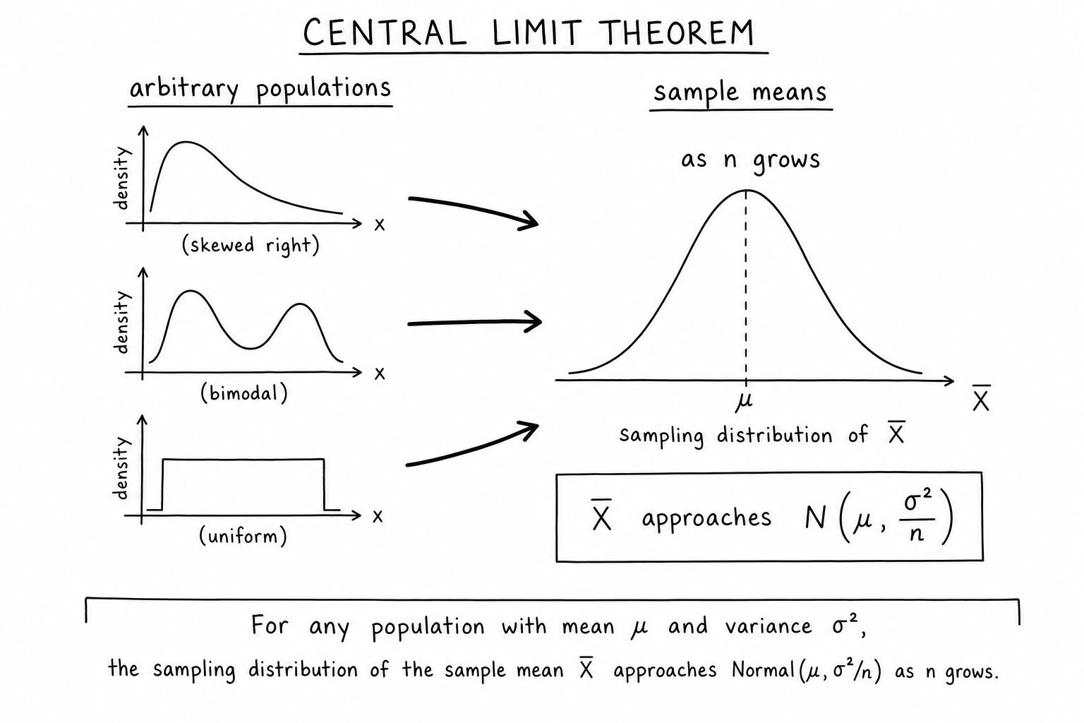
The Central Limit Theorem (CLT) is the reason classical statistics works. It says that when you average enough independent samples from almost any distribution, the average follows a normal distribution. The original data can be skewed, bimodal, uniform, or downright weird. The averages still converge to a bell curve.

This is what lets opinion polls publish margins of error from samples of a thousand people. It’s why A/B test calculators report z-scores. It’s the bridge between messy real data and the tidy normal-distribution toolkit. Understanding the central limit theorem changes how you read every statistic that comes from a sample.

This study note covers the formal statement, the intuition behind why it works, the rule-of-thumb sample size, several worked examples (polling, sample variance), the conditions where the CLT fails, and the way it underpins everyday inference, machine learning, and the entire idea of confidence intervals.

Central limit theorem distributions converging to normal modern textbook illustration

The Statement

Take $n$ independent and identically distributed (i.i.d.) random variables $X_1, X_2, \ldots, X_n$ with mean $\mu$ and finite variance $\sigma^2$. Their sample mean is:

$$\bar{X} = \frac{1}{n}\sum_{i=1}^{n} X_i$$

As $n$ grows large, the distribution of $\bar{X}$ approaches a normal distribution:

$$\bar{X} \xrightarrow{d} N\left(\mu, \frac{\sigma^2}{n}\right)$$

Two things to notice. The mean of the sampling distribution stays at $\mu$. The variance shrinks as $n$ grows — divided by sample size. That shrinking is why bigger samples give tighter estimates.

An equivalent statement: the standardized sample mean converges to a standard normal distribution:

$$\frac{\bar{X} – \mu}{\sigma / \sqrt{n}} \xrightarrow{d} N(0, 1)$$

This form is the foundation for z-tests, confidence intervals, and most parametric inference.

What ‘Large Enough’ Means

The classical rule of thumb is $n \geq 30$. For roughly symmetric distributions, even $n = 10$ is often fine. For heavily skewed distributions, you may need $n = 100$ or more before the sample mean looks normal.

The threshold depends on how far the underlying distribution sits from normal. Skewness and heavy tails slow convergence. Symmetric, light-tailed distributions converge fast. When in doubt, simulate it — generate samples and look at the histogram of means.

Specific guidance:

For approximately symmetric distributions: $n \geq 15$ usually suffices.
For mildly skewed distributions: $n \geq 30$ is the standard recommendation.
For strongly skewed (e.g., income, lognormal): $n \geq 50–100$ may be needed.
For extremely heavy tails: classic CLT may not apply at all.

Why It Works (Intuition)

Each sample contains its own random noise. When you average many samples together, positive and negative deviations cancel out. What remains is the underlying signal — the true mean — plus residual noise that gets smaller and more symmetric as $n$ grows.

The reason the residual is specifically normal traces back to how independent random variables combine. The normal distribution is a fixed point under averaging. Once a distribution is close to normal, averaging keeps it close to normal. The CLT formalizes that pull toward the bell curve.

A second intuition: Lyapunov’s version of the CLT shows that as long as no individual variable contributes a disproportionate share to the total, the sum is normal. Real-world quantities that arise as sums of many small independent influences (heights, measurement errors, sample averages) are normal for the same reason.

Worked Example: Polling

You poll 1,000 random voters and 52% support candidate A. Each voter is a binary trial with true (unknown) population proportion $p$. The sample proportion $\hat{p}$ has approximate distribution:

$$\hat{p} \sim N\left(p, \frac{p(1-p)}{n}\right)$$

Standard error: $\sqrt{0.52 \times 0.48 / 1000} \approx 0.0158$. The 95% margin of error is about $1.96 \times 0.0158 \approx \pm 3.1\%$. The poll says A is at 52%, but the true value is plausibly anywhere from 49% to 55%. That’s the CLT speaking.

Notice how the formula explains every poll headline you’ve ever read. Sample size 1,000 with proportions near 50% gives margin of error ≈ ±3%. That’s why most national polls report exactly that figure.

Worked Example: Sampling Distribution of the Mean

Suppose annual rainfall in a region is uniformly distributed between 30 and 70 cm. Mean = 50, variance = (70−30)² / 12 ≈ 133.3, σ ≈ 11.55.

If you average 25 years of rainfall, the sample mean has approximate distribution:

$$\bar{X} \sim N\left(50, \frac{133.3}{25}\right) = N(50, 5.33)$$

Standard error of the mean: √5.33 ≈ 2.31. So 95% of the time, the 25-year average rainfall falls within roughly 50 ± 4.6 cm.

The original distribution (uniform) looks nothing like a bell curve. The sampling distribution of the mean does. That’s the CLT making something useful out of messy raw data.

CLT vs Law of Large Numbers

The law of large numbers says sample means converge to the true mean as n grows: $\bar{X} \to \mu$. The CLT says how — describing the shape of the sampling distribution as approximately normal with variance $\sigma^2 / n$. LLN tells you you’ll get there; CLT tells you the road and the rate.

Together they form the foundation of most empirical statistics. LLN justifies estimating means from samples. CLT lets you put error bars on those estimates.

Where the CLT Quietly Breaks

Infinite or undefined variance. Cauchy and Pareto distributions with shape parameter ≤ 2 have variances that don’t exist. Sample means don’t converge to normal — they keep hopping around. Stable distributions (with exponent ≠ 2) are needed instead.
Strong dependence. CLT assumes independent samples. Time series with autocorrelation or clustered survey data violate this and need adjusted methods (block bootstrap, generalized least squares, sandwich estimators).
Tiny samples from heavy-tailed data. The CLT is asymptotic. Small $n$ from a fat-tailed distribution (like financial returns) leaves you with sample means that still look skewed and dangerous.
Non-identical distributions. Classical CLT requires i.i.d. data. Lyapunov and Lindeberg generalizations relax this but still require no individual variable dominating the total. Real-world cases where one observation matters disproportionately (extreme weather events, super-spreader infections) violate even the generalized versions.

The CLT is the reason most statistics works. It’s also the reason naive risk models miss tail events. Read more in the mathematics of risk assessment.

A Brief History

Abraham de Moivre proved the binomial-to-normal special case in 1733. Pierre-Simon Laplace generalized it in his 1812 Théorie analytique des probabilités. The modern general statement and rigorous proofs came in the early 20th century from Aleksandr Lyapunov (1901) and Jarl Waldemar Lindeberg (1922). Pólya named the result the “central limit theorem” in 1920, with “central” referring to its centrality to probability theory rather than to centering values around a mean.

The CLT remained somewhat theoretical until computers made it possible to verify it empirically and to build resampling methods (bootstrap, Monte Carlo) that lean on its conclusions. Today the CLT underpins almost every confidence interval, hypothesis test, and Bayesian normal approximation in applied statistics.

Why It Matters in Practice

Polling and surveys. Margins of error are CLT-derived.
A/B testing. Standard error of the difference between two sample means uses CLT.
Quality control. Control charts assume sample means follow approximate normality.
Manufacturing tolerances. Stack-up analysis treats accumulated random errors as approximately normal.
Finance. Diversified portfolio returns become approximately normal even when individual stocks aren’t, because they’re sums of many partial contributions.
Bootstrap and resampling. The bootstrap distribution converges to the true sampling distribution under conditions related to CLT validity.
Machine learning. Stochastic gradient descent’s convergence properties leverage CLT-like reasoning. The central limit theorem is also why sums of random initialization weights behave nicely in neural networks.

Lyapunov vs Lindeberg Conditions

The classical CLT requires i.i.d. samples. Lyapunov’s CLT (1901) and Lindeberg’s CLT (1922) generalize it to independent but not identically distributed variables, provided no individual variable contributes a disproportionate share of the total variance.

The Lindeberg condition asks: as $n$ grows, does the contribution of any single variable to the total become negligible? If yes, the sum is asymptotically normal. This justifies treating real-world quantities — heights, measurement errors, polling aggregates — as approximately normal even when the underlying variables aren’t identically distributed.

The Lyapunov condition is similar but uses a moment condition ($2 + \delta$ moments must exist for some $\delta > 0$). It’s slightly stronger but easier to verify in some applications.

Bootstrap and Resampling Methods

The bootstrap (Efron, 1979) is a resampling method that approximates the sampling distribution of a statistic by repeatedly drawing samples (with replacement) from the observed data. It works because of CLT-like reasoning: the distribution of bootstrap statistics converges to the true sampling distribution under regularity conditions related to the CLT.

Bootstrap confidence intervals don’t require normality assumptions and work for many statistics where classical CLT-based methods are unavailable (medians, quantiles, complex composite statistics). Modern statistical practice uses bootstrap routinely for inference, especially when sample sizes are small or distributions are unusual.

Monte Carlo Simulation as Empirical CLT

Monte Carlo methods simulate complex systems by repeatedly sampling input distributions and aggregating results. The averages and confidence intervals from Monte Carlo runs follow the CLT — sample means of simulation outcomes are normally distributed with standard error $\sigma / \sqrt{n}$.

This is why Monte Carlo standard errors shrink slowly: doubling precision requires quadrupling the number of simulations. It also justifies the standard practice of reporting Monte Carlo results with $\pm$ standard errors derived directly from the CLT.

Worked Example: Quality Control

A factory produces bolts with mean diameter 10 mm and standard deviation 0.5 mm. The underlying distribution is roughly uniform over [9, 11], not normal. Quality control samples 50 bolts per shift and computes the mean.

By the CLT, the sample mean has approximate distribution:

$$\bar{X} \sim N\left(10, \frac{0.25}{50}\right) = N(10, 0.005)$$

Standard error: $\sqrt{0.005} \approx 0.071$ mm. Control chart limits at ±3 standard errors give an alarm threshold of $10 \pm 0.213$ mm. Sample means outside that range trigger investigation. The CLT lets quality engineers use normal-distribution control chart math even though the underlying bolt diameter distribution isn’t normal.

CLT and the Standard Error

Standard error of the mean = $\sigma / \sqrt{n}$. This formula falls directly out of the CLT: the sampling distribution variance is $\sigma^2 / n$, so the standard deviation (which is what “standard error” means) is the square root.

Three implications:

To halve standard error, you need to quadruple sample size. Precision is expensive at the margin.
The CLT gives the same standard-error formula regardless of the underlying distribution shape (as long as variance is finite).
For non-normal data with finite variance, the standard-error formula is still valid; only the normality of the sampling distribution requires CLT to kick in.

CLT in the Bootstrap World

Bootstrap methods (Efron, 1979) estimate sampling distributions by resampling with replacement from observed data. The bootstrap distribution converges to the true sampling distribution as both $n$ and the number of bootstrap replicates grow. The convergence relies on CLT-like reasoning at its core.

For statistics other than the mean (medians, quantiles, ratios, regression coefficients), classical CLT may not apply directly, but the bootstrap usually still works. This is why modern statistical practice often defaults to bootstrap inference for complex statistics — it sidesteps the need to derive a CLT result by hand.

Continuous Distributions, Discrete Distributions, and the CLT

The CLT applies to both discrete and continuous random variables. The classic illustration uses dice: roll one die and the distribution of outcomes is uniform on {1,…,6}. Roll many dice and average the results, and the distribution of the mean approaches normal.

Even with as few as 10 dice, the sample mean distribution is visibly bell-shaped. With 30 dice, it’s nearly indistinguishable from normal. This is the simplest hands-on demonstration of the CLT and is the basis for many introductory statistics simulations.

Why the Theorem Is Called ‘Central’

The “central” in central limit theorem doesn’t refer to centering values around a mean. It comes from the German word zentral, used by George Pólya in 1920 to convey that this result is central to probability theory — meaning fundamentally important and foundational. The terminology stuck even though it sometimes confuses students who assume “central” refers to the geometric centering of a distribution.

Among limit theorems in probability, the CLT earns the “central” label because it underlies almost every classical inference procedure, every confidence interval, and most of statistical theory built before computational methods became practical.

Worked Example: Coin Flips

Flip a fair coin 100 times. Each flip is a Bernoulli trial with mean 0.5 and variance 0.25. The number of heads follows a binomial distribution with mean 50 and variance 25 (standard deviation 5).

By the CLT, the count of heads is approximately normal: $X \sim N(50, 25)$. The probability of getting between 40 and 60 heads is approximately $P(-2 < Z < 2) \approx 0.954$ — a tight band around 50 that holds 95% of all outcomes.

Without the CLT you’d compute this probability as a sum of binomial coefficients, which is doable but tedious. With the CLT it’s a one-line z-score lookup. This is the simplest practical demonstration of why the CLT is so useful: it converts hard combinatorial calculations into easy normal-distribution lookups.

CLT and Sampling Distribution Convergence Speed

How fast the sample mean distribution converges to normal depends on three factors: sample size, the shape of the underlying distribution, and what statistic you’re computing.

For symmetric, light-tailed distributions: convergence is fast. Even $n = 10$ often produces near-normal sample mean distributions.
For moderately skewed distributions: $n = 30$ (the textbook rule) is usually adequate.
For heavily skewed or heavy-tailed distributions: $n = 100$ or more may be needed before the bell shape emerges.
For statistics other than the mean (medians, ratios, regression coefficients): convergence rates and conditions differ, often requiring larger samples or specialized arguments.

The Berry-Esseen theorem provides a quantitative bound on convergence speed for the mean, expressing the maximum error in normal approximation as a function of sample size and the third moment of the distribution. Skewness slows the convergence linearly with the third moment.

FAQs

What does the Central Limit Theorem actually say?

The distribution of the sample mean approaches a normal distribution as the sample size grows, regardless of the shape of the underlying distribution — provided the underlying distribution has a finite variance and the samples are independent.

How large does the sample need to be for the CLT to apply?

There’s no universal cutoff. n ≥ 30 is the textbook rule of thumb. Symmetric, light-tailed distributions converge faster. Heavily skewed or heavy-tailed distributions may need n in the hundreds. Simulating sampling distributions is the cleanest check.

Does the Central Limit Theorem apply to any distribution?

It applies to any distribution with finite variance and independent samples. It fails for distributions with infinite variance (Cauchy, Pareto with shape ≤ 2) and for samples that aren’t independent.

What’s the difference between the CLT and the law of large numbers?

The law of large numbers says sample means converge to the true mean as n grows. The CLT says how — describing the shape of the sampling distribution as approximately normal with variance σ²/n. LLN tells you you’ll get there; CLT tells you the road.

Why does the CLT matter in practice?

It’s the foundation of most parametric inference: confidence intervals, hypothesis tests, regression standard errors, A/B test analysis. Any time you build a margin of error from a sample mean, you’re trusting the CLT to make the math valid.

Does the CLT apply to medians and other statistics?

There are CLT-like results for medians, quantiles, and many other statistics, but the convergence rates and limiting distributions differ from the simple sample-mean case. The bootstrap is the modern catch-all when classical CLT results don’t directly apply.

What’s the standard error of the mean?

It’s the standard deviation of the sampling distribution of the mean: SE = σ / √n. The CLT says the sample mean is approximately normal with this standard error, which is why bigger samples give tighter estimates and why standard error shrinks with √n, not n.

How is the CLT used in A/B testing?

When you compare conversion rates between two variants, the difference in sample proportions is approximately normal by the CLT. That lets you compute z-scores, p-values, and confidence intervals directly from sample means and standard errors. Tools like Optimizely, VWO, and Statsig all rely on this.

Can the CLT explain why so many real-world variables look normal?

Partially. Many natural quantities (heights, measurement errors, biological traits) arise as sums of many small independent influences, which the CLT predicts will be approximately normal. The ‘normal because additive’ explanation is the central reason the bell curve shows up everywhere in nature.

What’s a stable distribution and how does it generalize the CLT?

Stable distributions are the limiting distributions of sums of i.i.d. random variables when variance is infinite. The normal distribution is the special case with stability index α = 2. For α < 2, the limit is a heavy-tailed stable distribution. This is the right framework for genuinely fat-tailed data, including some financial returns.

Why is the rate of convergence in CLT slow for skewed distributions?

Because the sampling distribution of skewed-data sample means takes longer to lose its skewness. The Berry-Esseen theorem quantifies the convergence rate: error in normal approximation is bounded by C × (third moment) / (σ³ √n). Skewed distributions have large third moments, slowing convergence.

Does CLT apply to maxima and minima?

Not directly. The distribution of sample maxima is governed by extreme value theory (Gumbel, Fréchet, Weibull distributions), not the normal distribution. The CLT is specifically about sums and averages; tails follow different limit laws.

How is the CLT related to the standard error formula?

The CLT directly produces the formula SE = σ/√n for the standard error of the sample mean. The sampling distribution variance is σ²/n; standard error is its square root. This formula holds regardless of the underlying distribution shape (assuming finite variance), which is why it’s the universal foundation for confidence intervals.