
 by
by
A single glass of water holds about 1025 molecules. To predict its behavior from first principles, you’d have to write Newton’s equations of motion for every one of them and solve the whole set simultaneously. No computer on Earth can do that. No computer we’ll ever build can do that.
Statistical mechanics gets around this with a trick that feels almost like cheating. Instead of following one system’s 1025 particles through time, you imagine an enormous collection of mental copies of the system, every copy prepared under the same macroscopic conditions, and you average over the copies. That imaginary collection is called an ensemble.
The idea comes from J. Willard Gibbs, who built statistical mechanics around it in his 1902 book Elementary Principles in Statistical Mechanics. And it trips up almost everyone at first: why would imagining copies of a system tell you anything about the one real system sitting in front of you? Hold that question. The answer arrives with the ensemble average near the end, and it’s satisfying.
Table of Contents
What Is an Ensemble in Statistical Mechanics?
An ensemble is a collection of a very large number of macroscopically identical but essentially independent systems. Both halves of that definition carry weight, so take them one at a time.
Macroscopically identical means every copy satisfies the same bulk conditions: the same volume \( V \), pressure \( P \), temperature \( T \), energy \( E \), or particle number \( N \), whichever of these the ensemble holds fixed. Measure any macroscopic property and you couldn’t tell two copies apart.
Essentially independent means the systems don’t interact with each other. Microscopically, no two copies are alike. One has a particular molecule near the wall, another has it dead center. The copies differ in quantum states, parity, symmetry, in every microscopic detail that a bulk measurement can’t see.
That’s the whole construction: one macrostate, realized by an astronomical number of different microstates. If the macrostate vs microstate distinction feels fuzzy, read my post on macrostates, microstates and thermodynamic probability first. Ensembles sit directly on top of it.
Types of Ensembles
There are three standard ensembles, and the classification comes down to a single question: what is each system allowed to exchange with its neighbors? Nothing at all, energy only, or energy and particles both.
- Micro-canonical ensemble: exchanges nothing. Energy \( E \), volume \( V \) and particle number \( N \) stay fixed.
- Canonical ensemble: exchanges energy. Temperature \( T \), volume \( V \) and particle number \( N \) stay fixed.
- Grand canonical ensemble: exchanges energy and particles. Temperature \( T \), volume \( V \) and chemical potential \( \mu \) stay fixed.
The walls between the systems enforce these rules. Watch the walls in the figures below and the three definitions become hard to forget: every adjective on a wall (rigid, impermeable, insulated, conducting, permeable) locks or unlocks one physical quantity.
Micro-canonical Ensemble
The micro-canonical ensemble is the collection of systems that all share the same energy E, volume V and total number of particles N. Each system is completely isolated. Nothing gets in, nothing gets out.
The walls make that isolation concrete. Every system is separated by rigid, impermeable, insulated walls. Rigid, so the volume can’t change. Impermeable, so particles can’t pass. Insulated, so heat can’t flow. Three adjectives, three locked quantities.
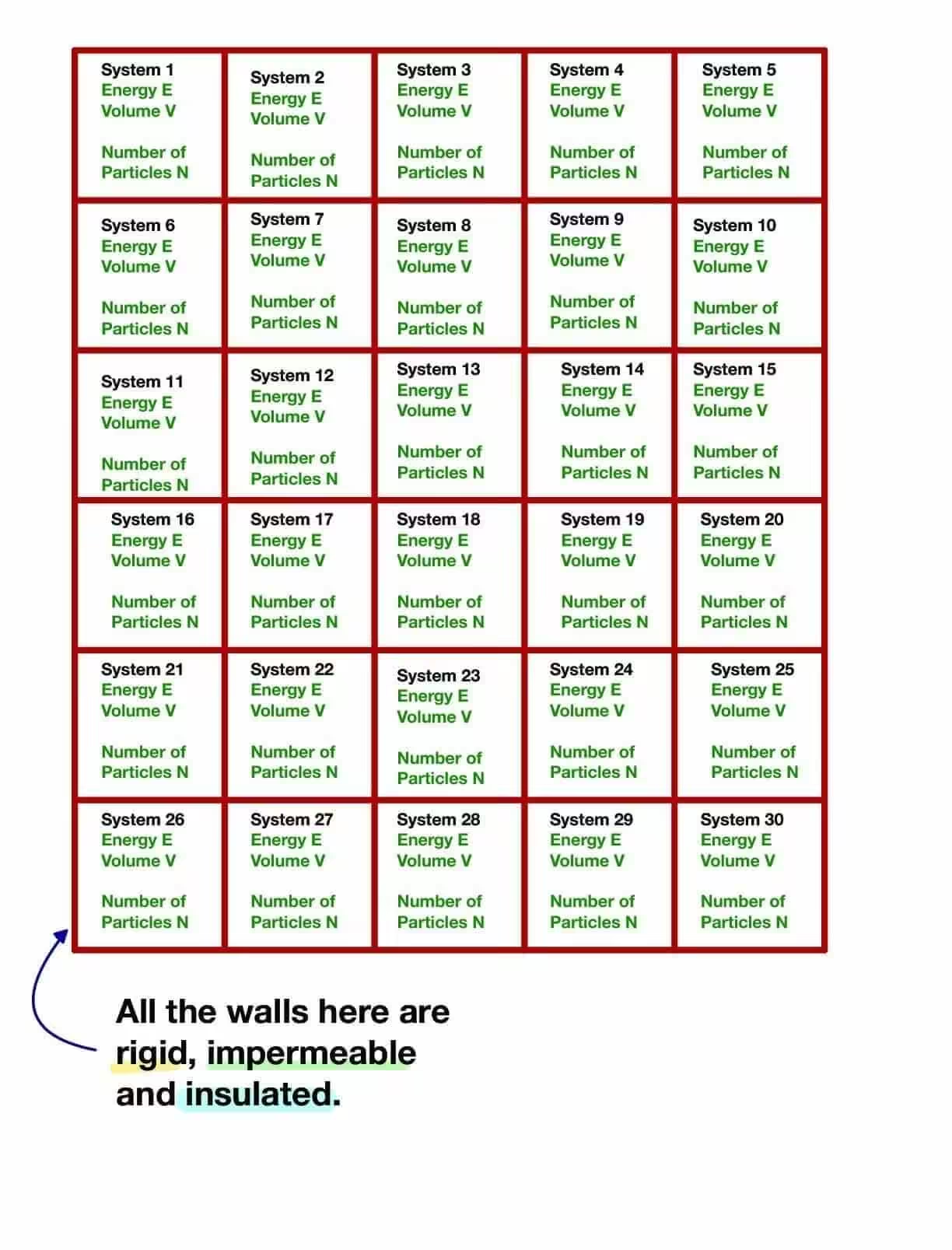
Here all the borders are impermeable and insulated.
The central quantity in this ensemble is \( \Omega(E, V, N) \), the count of microstates available to a system at energy \( E \). Boltzmann’s entropy formula turns that count into thermodynamics:
$$ S = k_B \ln \Omega $$
where \( k_B = 1.38 \times 10^{-23} \, \mathrm{J/K} \) is Boltzmann’s constant. Count the microstates, take the logarithm, and you have entropy. Temperature, pressure and the rest follow from derivatives of \( S \), exactly as the laws of thermodynamics demand.
One catch that textbooks mention too late: the micro-canonical ensemble is conceptually the cleanest of the three and computationally the ugliest. Counting states at exactly energy \( E \) is hard even for toy models. That pain is why the next ensemble exists.
Canonical Ensemble
The canonical ensemble is the collection of systems sharing the same temperature T, volume V and number of particles N. Energy is no longer fixed. Each system trades heat with its neighbors.
Equal temperature is achieved by thermal contact: the internal walls are rigid and impermeable but conducting. The outer wall of the whole ensemble stays insulated and impermeable, so the collection as a whole is isolated even though its members constantly exchange heat.
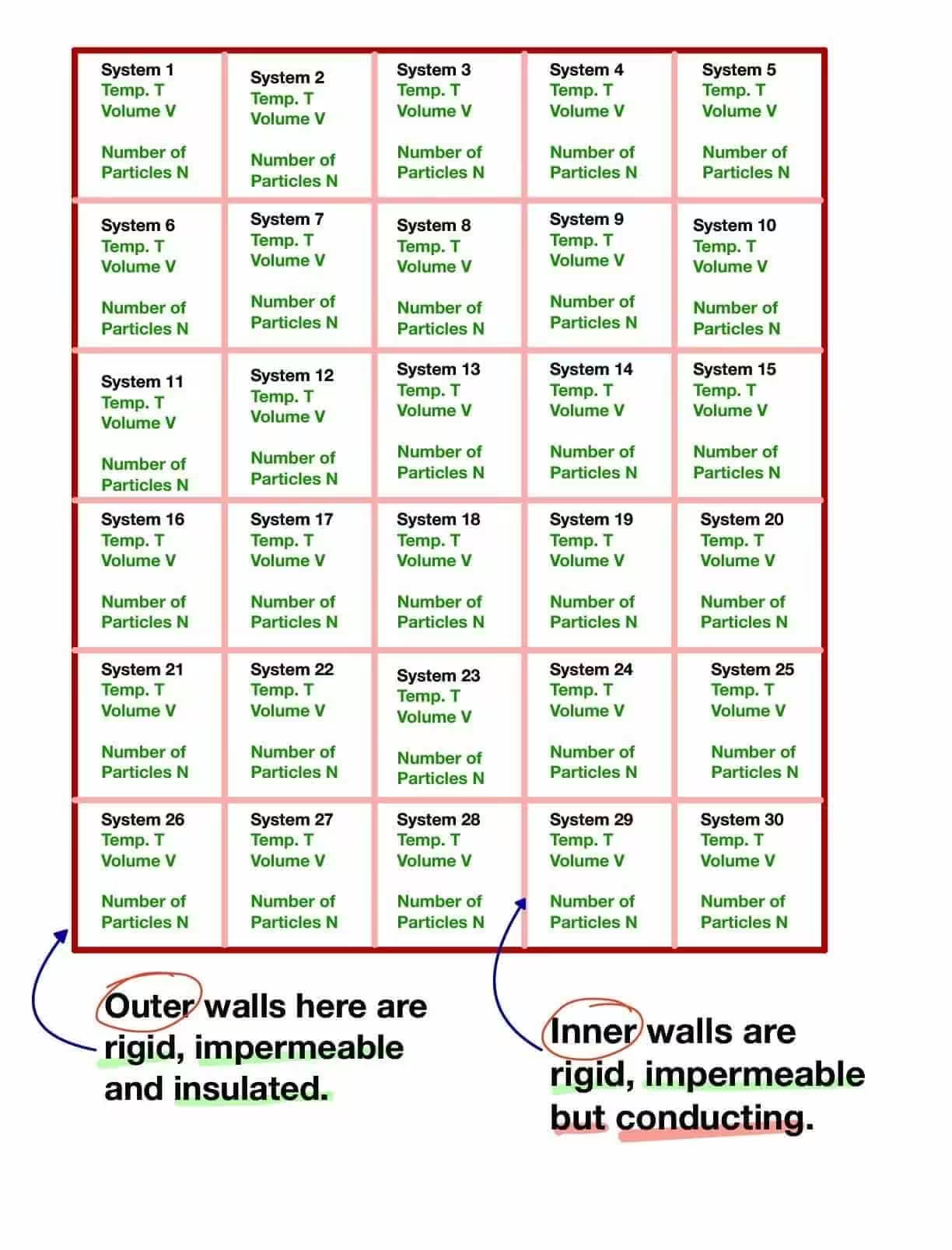
Here, the borders in bold shade are both insulated and impermeable, while the borders in light shade are conducting and impermeable.
Because heat flows, a system’s energy fluctuates around an average. The probability of finding a system in a microstate \( i \) with energy \( E_i \) follows the Boltzmann distribution:
$$ P_i = \frac{e^{-E_i / k_B T}}{Z}, \qquad Z = \sum_i e^{-E_i / k_B T} $$
\( Z \) is the partition function, and it’s the workhorse of the entire subject. It looks like a bookkeeping device (it’s literally the normalization constant of the probabilities), yet free energy, entropy, pressure and heat capacity all drop out of derivatives of \( \ln Z \).
But wait: if energy fluctuates, how can this describe a lab sample with a perfectly steady thermometer reading? Because the fluctuations are absurdly small. Relative energy fluctuations scale as \( 1/\sqrt{N} \). For \( N \approx 10^{23} \), that’s about one part in 300 billion. No instrument you’ll ever touch can resolve it.
Grand Canonical Ensemble
The grand canonical ensemble is the collection of systems sharing the same temperature T, volume V and chemical potential \( \mu \). Now both energy and particles flow between systems.
Chemical potential deserves a plain translation: \( \mu \) is the energy cost of adding one more particle to the system. Heat flows down a temperature gradient; particles flow down a chemical potential gradient. Equal \( \mu \) everywhere means no net particle flow, the same way equal \( T \) means no net heat flow.
The systems of a grand canonical ensemble are separated by rigid, permeable and conducting walls, while the outer borders stay impermeable and insulated.
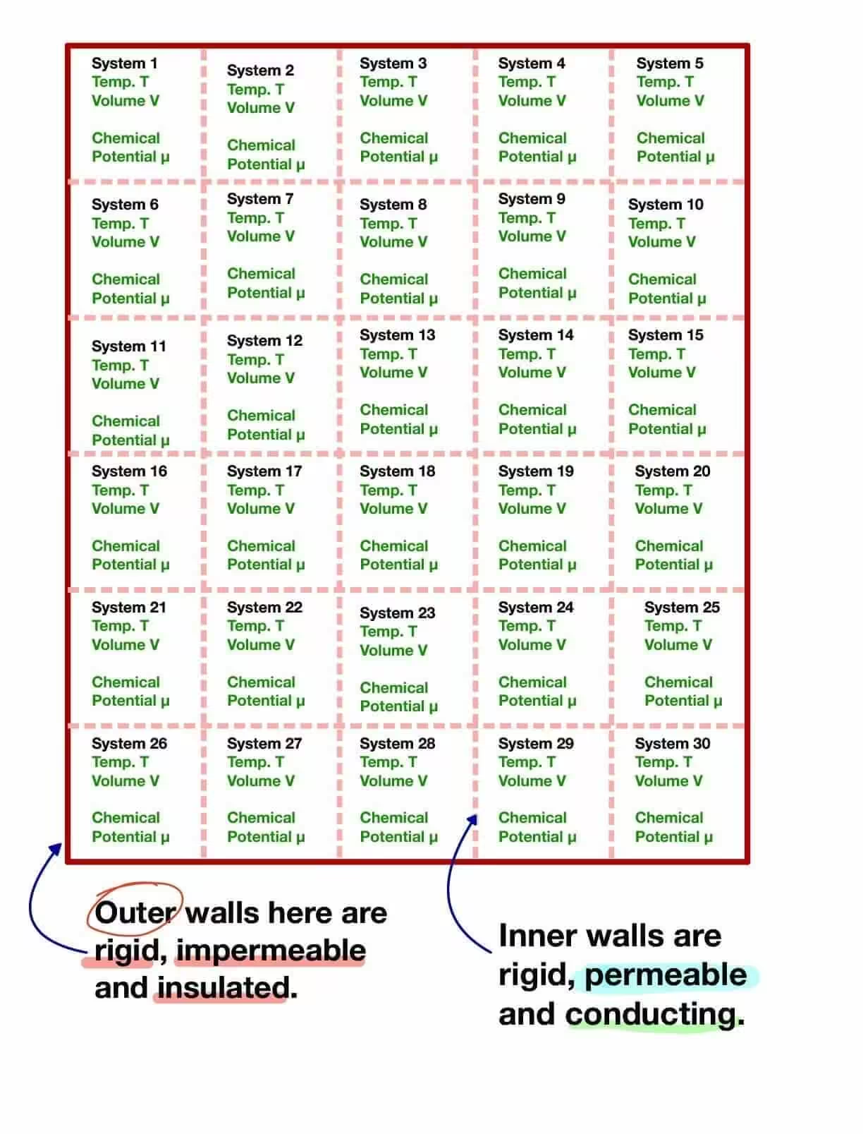
Exchange of heat and particles continues until every system settles at the common temperature \( T \) and common chemical potential \( \mu \).
The bookkeeping generalizes too. The grand partition function sums over states of every possible particle number:
$$ \mathcal{Z} = \sum_i e^{-(E_i – \mu N_i)/k_B T} $$
If that looks like an unnecessary complication, here’s the payoff: the grand canonical ensemble is where quantum statistics live. The Fermi-Dirac and Bose-Einstein distributions, electrons in metals, photons in blackbody radiation (the same physics that produced Wien’s laws and, eventually, quantum theory), all of them fall out of \( \mathcal{Z} \) in half a page. Deriving them canonically is a genuine slog.
Micro-canonical vs Canonical vs Grand Canonical
Every distinction from the last three sections fits in one table. If you memorize nothing else from this lesson, memorize the first two rows.
| Micro-canonical | Canonical | Grand canonical | |
|---|---|---|---|
| Held fixed | E, V, N | T, V, N | T, V, μ |
| Exchanges | Nothing | Energy | Energy + particles |
| Inner walls | Rigid, impermeable, insulated | Rigid, impermeable, conducting | Rigid, permeable, conducting |
| Fluctuates | Nothing | Energy | Energy and N |
| Key function | Ω, via S = kB ln Ω | Partition function Z | Grand partition function |
| Best for | Foundations, isolated systems | Lab systems at fixed T | Quantum gases, open systems |
One fact makes the whole choice less stressful than it looks: in the thermodynamic limit (\( N \to \infty \) at fixed density), all three ensembles predict identical thermodynamics. The fluctuations that distinguish them vanish as \( 1/\sqrt{N} \). So you pick an ensemble by computational convenience, never by physical necessity. That’s the whole secret of ensemble choice.
Ensemble Average
Here’s the payoff of the entire construction, and the answer to the question from the top. A macroscopic measurement never sees one microstate. A thermometer takes milliseconds; molecules collide every picosecond. Every reading you’ve ever taken is a time average over billions of microstates.
Time averages over 1023 interacting particles are hopeless to compute. Ensemble averages aren’t. So statistical mechanics swaps one for the other: average over the copies instead of over time.
Picture phase space, the space whose coordinates are every position and every momentum in the system. Each member of the ensemble is a single point in it. Let \( R(x) \) be a statistical quantity along the x-axis and \( N(x) \) be the number of phase points in phase space, then the ensemble average of the statistical quantity \( R \) is defined as,
$$ \bar{R} := \dfrac{\int_{-\infty}^{\infty} R(x) N(x) \, \mathrm{d}x}{\int_{-\infty}^{\infty} N(x) \, \mathrm{d}x} $$
Read it as a weighted mean: regions of phase space crowded with ensemble members count more, empty regions count less. The denominator just normalizes the weights.
The quiet assumption underneath the swap is called the ergodic hypothesis: a single system, evolving long enough, visits all the microstates that the ensemble’s copies occupy, so the time average equals the ensemble average. It’s plausible, and it works spectacularly well. But after more than a century, it remains unproven for most realistic systems. Verification isn’t proof, and this is one of the live edges of the subject.
Downloads
Enter your email and I’ll send the PDF straight to your inbox. Free and print-friendly.
Recommended Books on Statistical Physics
These are the texts this lesson leans on, with current prices. If you want full reviews and a reading order before buying, I ranked them in my guide to the best statistical mechanics books.
FAQs on Ensembles
What is an ensemble in statistical mechanics?
An ensemble is a collection of a very large number of imaginary copies of a system, all prepared under identical macroscopic conditions but differing in microscopic detail. J. Willard Gibbs introduced the concept in 1902. Averaging a quantity over the copies reproduces what you’d measure on the one system in your lab.
What is the difference between microcanonical, canonical and grand canonical ensembles?
The difference is what each system can exchange with its surroundings. Microcanonical systems exchange nothing (fixed E, V, N). Canonical systems exchange energy only (fixed T, V, N). Grand canonical systems exchange both energy and particles (fixed T, V, and chemical potential).
Why do we need ensembles at all?
Because a macroscopic system holds around 10 to the power 23 particles, and solving equations of motion for each one is impossible. Ensembles replace that impossible calculation with an average over copies, which turns out to match what thermometers and pressure gauges actually measure.
Which ensemble should I use for a given problem?
Pick by convenience, not by principle. Use the canonical ensemble for anything held at fixed temperature, which covers most laboratory systems. Use the grand canonical ensemble for quantum gases and open systems where particle number varies. The microcanonical ensemble mostly serves foundations and isolated idealizations.
Do the three ensembles give the same answers?
For large systems, yes. In the thermodynamic limit, relative fluctuations shrink as one over the square root of N, so all three ensembles predict identical thermodynamic quantities. They only disagree for very small systems, like nanoclusters or single molecules, where fluctuations are comparable to averages.
What is the ensemble average?
The ensemble average is the mean value of a physical quantity computed over all members of the ensemble, weighted by how densely the systems populate each region of phase space. Under the ergodic hypothesis, it equals the time average you’d measure on a single system.
What is the ergodic hypothesis?
The ergodic hypothesis says that a single system, left to evolve long enough, passes through all the microstates that the ensemble’s copies occupy. That’s what lets you swap a time average for an ensemble average. It’s widely assumed and works extremely well, but it remains unproven for most realistic systems.
Tell Google you want more of this.
Add Gaurav Tiwari as a preferred sourceOne tap, and this site shows up more often in your own Top Stories, AI Overviews and AI Mode. Remove it any time.
Disclaimer: This site is reader-supported. If you buy through some links, I may earn a small commission at no extra cost to you. I only recommend tools I trust and would use myself. Your support helps keep gauravtiwari.org free and focused on real-world advice. Thanks. - Gaurav Tiwari