Zero of a Function

The zero of a function is the input value that makes the output equal to zero. You’ll encounter this concept constantly, from basic algebra through calculus and beyond. Every time you solve an equation like \( f(x) = 0 \), you’re hunting for zeroes.

Zeroes aren’t just an abstract classroom exercise. If you’re calculating a break-even point for a business, modeling projectile motion, or finding where two curves intersect, you’re solving for zeroes. The skill transfers directly to real-world problem solving.

In this guide, you’ll learn:

• What a function’s zero actually represents and why it matters.
• How to find zeroes for quadratic, polynomial, rational, and other common functions.
• How to read zeroes directly from a function’s graph.
• Numerical methods like Newton-Raphson and bisection for approximating zeroes.
• Real-world applications in calculus, engineering, and physics.

Let’s start with the definition and build from there.

What is the zero of a function?

A zero of a function \( f \) is any value \( x = a \) where \( f(a) = 0 \). On a graph, these are the points where the curve crosses or touches the x-axis. The point \( (a, 0) \) is called an x-intercept, and the value \( a \) itself is the zero.

Here are a few quick examples so you can see the pattern:

• The function \( f(x) = x + 1 \) has a zero at \( x = -1 \), because \( f(-1) = -1 + 1 = 0 \).
• The function \( g(x) = x^2 – 4 \) has two zeroes: \( x = -2 \) and \( x = 2 \), since \( g(-2) = 0 \) and \( g(2) = 0 \).
• If the graph of \( h(x) \) passes through \( (-3, 0) \), then \( x = -3 \) is a zero of \( h(x) \).

On a graph, you can spot real zeroes by looking at where the curve meets the x-axis. But keep in mind that not every function’s zeroes are visible on the graph. Some zeroes are complex numbers (involving \( i \)), which means the graph never actually crosses the x-axis. The function still has zeroes; you just can’t see them on a standard coordinate plane.

Understanding the zero of a function is foundational to function notation and rules. Once you’re comfortable with what zeroes mean, the algebraic techniques below will feel much more intuitive.

How to find the zeroes of a function

The core method is straightforward: set \( f(x) = 0 \) and solve for \( x \). What changes from problem to problem is the technique you use to solve that equation.

For a linear function like \( f(x) = 3x – 9 \), you simply isolate \( x \) to get \( x = 3 \). This is the same process you’d use when solving linear equations. For more involved expressions, you might need factoring, the quadratic formula, synthetic division, or numerical methods. The difficulty scales with the complexity of the function, but the starting point is always the same: make the function equal zero and work from there.

Zeroes of a quadratic function

Quadratic functions deserve special attention because so many higher-degree problems eventually reduce to them. Once you’re comfortable finding zeroes of quadratics, you’ll handle a huge portion of algebra problems with confidence.

To find the zeroes of a quadratic \( ax^2 + bx + c = 0 \), keep these points in mind:

• A quadratic function has at most two zeroes.
• Always rewrite the equation in standard form \( ax^2 + bx + c = 0 \) before solving.
• Try factoring first. If that doesn’t work cleanly, use the quadratic formula \( x = \frac{-b \pm \sqrt{b^2 – 4ac}}{2a} \).

The table below helps you pick the right strategy:

Guide question	Strategy
Is the quadratic expression factorable?	Factor and set each factor equal to zero.
Is the expression not easily factorable?	Apply the quadratic formula.
Does it match a special pattern (perfect square trinomial or difference of squares)?	Use the corresponding identity to factor directly.

The discriminant tells you what to expect

Before you even start solving, the discriminant \( \Delta = b^2 – 4ac \) reveals how many real zeroes a quadratic has. If \( \Delta > 0 \), you’ll get two distinct real zeroes. If \( \Delta = 0 \), there’s exactly one real zero (a repeated root). And if \( \Delta < 0 \), both zeroes are complex, so the parabola never crosses the x-axis.

For example, \( x^2 – 5x + 6 = 0 \) factors as \( (x-2)(x-3) = 0 \), giving zeroes at \( x = 2 \) and \( x = 3 \). The discriminant here is \( 25 – 24 = 1 > 0 \), confirming two distinct real roots. If you had \( x^2 + x – 1 = 0 \) instead, factoring won’t produce integer roots, so you’d reach for the quadratic formula. Any solid calculus textbook covers these methods in detail with worked examples.

Zeroes of a polynomial function

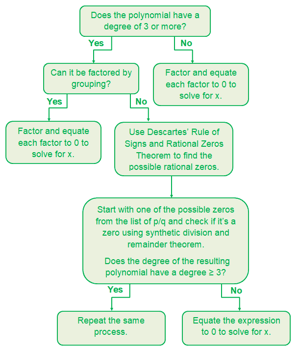
For polynomials of degree three or higher, the process builds on everything you already know about quadratics. Set the polynomial equal to zero, then look for ways to break it down into simpler factors.

You can use the Rational Root Theorem to generate a list of possible rational zeroes, then test them with synthetic division. Each time you find a zero, you reduce the polynomial’s degree by one. Eventually you’ll reach a quadratic that you can solve with the methods above. The flowchart below summarizes this approach.

Multiplicity of zeroes

When a factor appears more than once, that zero has a multiplicity greater than one. For \( f(x) = (x – 2)^3(x + 1) \), the zero at \( x = 2 \) has multiplicity 3, and the zero at \( x = -1 \) has multiplicity 1.

Multiplicity affects graph behavior. Odd multiplicity means the curve crosses the x-axis at that zero. Even multiplicity means the curve touches the axis and bounces back. A zero of multiplicity 3 produces a distinctive flattening effect as the graph passes through the x-axis, which you can spot visually.

Zeroes of a rational function

A rational function has the form \( f(x) = \frac{p(x)}{q(x)} \), where both \( p(x) \) and \( q(x) \) are polynomials. To find its zeroes, you set the numerator equal to zero: \( p(x) = 0 \). Any solution that doesn’t also make the denominator zero is a valid zero of the function.

This extra check matters. If a value makes both the numerator and denominator zero, it creates a hole in the graph rather than an x-intercept. Always verify that your candidate zeroes don’t produce \( q(x) = 0 \) as well.

Zeroes of other common functions

The same principle, set the function equal to zero and solve, applies to every type of function you’ll encounter. The algebra changes, but the logic stays identical. Here are some function types you should be familiar with:

Type of function	Example	Finding the zero
Logarithmic	\( f(x) = \log_2(2x) \)	Set \( \log_2(2x) = 0 \), so \( 2x = 1 \), giving \( x = \frac{1}{2} \).
Power	\( f(x) = 3x^{1/3} \)	Set \( 3x^{1/3} = 0 \), giving \( x = 0 \).
Exponential	\( f(x) = 2^{x+1} – 4 \)	Set \( 2^{x+1} = 4 \), so \( x + 1 = 2 \), giving \( x = 1 \).
Trigonometric	\( f(x) = \sin(x) \)	Zeroes at \( x = n\pi \) for every integer \( n \).

For each of these, the real zeroes show up as x-intercepts on the graph. Trigonometric functions are especially interesting because they have infinitely many zeroes due to their periodic nature. If you’re working with trig zeroes, having a solid grasp of trigonometric identities will speed up the process considerably.

Graphical interpretation of zeroes

Graphs give you a visual shortcut for understanding the zero of a function. Instead of crunching algebra, you can look at where the curve hits the x-axis and read off approximate values. This is especially useful for confirming algebraic solutions or getting quick estimates.

There are three distinct behaviors to watch for at a zero:

• Crossing. The curve passes straight through the x-axis. This happens at zeroes with odd multiplicity (1, 3, 5, etc.).
• Touching (bouncing). The curve touches the x-axis and reverses direction. This happens at zeroes with even multiplicity (2, 4, 6, etc.).
• Flattening. At higher multiplicities (3+), the curve flattens noticeably as it passes through the zero, creating an inflection-like shape.

The Intermediate Value Theorem (IVT) provides a more rigorous graphical tool. If \( f(a) \) and \( f(b) \) have opposite signs, and \( f \) is continuous on \( [a, b] \), then there’s at least one zero between \( a \) and \( b \). You can use this to narrow down zero locations by evaluating the function at different points and watching for sign changes.

For example, if \( f(1) = -3 \) and \( f(2) = 5 \), continuity guarantees a zero somewhere between \( x = 1 \) and \( x = 2 \). Graphing calculators like the TI-84 or software like Desmos and GeoGebra can pinpoint these crossings to several decimal places using built-in root-finding features.

Numerical methods for finding zeroes

Not every equation can be solved with algebra. When you’re dealing with functions like \( f(x) = x – \cos(x) \) or \( f(x) = e^x – 3x \), there’s no neat formula to isolate \( x \). That’s where numerical methods come in. These algorithms approximate the zero of a function to whatever precision you need.

Bisection method

The bisection method is the simplest numerical approach. It relies on the Intermediate Value Theorem. You start with two points \( a \) and \( b \) where the function has opposite signs, then repeatedly halve the interval.

Here’s the procedure step by step:

1. Pick \( a \) and \( b \) such that \( f(a) \) and \( f(b) \) have opposite signs.
2. Compute the midpoint \( m = \frac{a + b}{2} \).
3. Evaluate \( f(m) \). If \( f(m) = 0 \), you’ve found the zero.
4. If \( f(m) \) has the same sign as \( f(a) \), replace \( a \) with \( m \). Otherwise, replace \( b \) with \( m \).
5. Repeat until the interval is smaller than your desired tolerance.

The bisection method is reliable but slow. Each iteration only halves the error, so reaching 6-decimal accuracy from an initial interval of width 1 takes about 20 iterations. It always converges though, which makes it a dependable fallback.

Newton-Raphson method

The Newton-Raphson method is faster and more widely used in practice. It uses the function’s derivative to make progressively better guesses. Starting from an initial estimate \( x_0 \), each iteration applies the formula:

\( x_{n+1} = x_n – \frac{f(x_n)}{f'(x_n)} \)

Geometrically, you’re drawing the tangent line at the current point and finding where it crosses the x-axis. That crossing becomes your next guess. When the initial estimate is close to the actual zero, Newton-Raphson converges quadratically, meaning the number of correct digits roughly doubles with each step.

Consider \( f(x) = x^2 – 2 \), which has a zero at \( \sqrt{2} \approx 1.41421 \). Starting with \( x_0 = 1 \):

• \( x_1 = 1 – \frac{1 – 2}{2(1)} = 1.5 \)
• \( x_2 = 1.5 – \frac{2.25 – 2}{2(1.5)} = 1.41667 \)
• \( x_3 = 1.41422 \) (already accurate to 5 decimal places)

Just 3 iterations to reach 5 correct decimals. That’s the power of quadratic convergence.

Secant method

The secant method is a variation of Newton-Raphson that doesn’t require computing the derivative. Instead, it approximates the derivative using two previous points:

\( x_{n+1} = x_n – f(x_n) \cdot \frac{x_n – x_{n-1}}{f(x_n) – f(x_{n-1})} \)

This is useful when the derivative is expensive or difficult to compute. The convergence rate is superlinear (roughly 1.618, the golden ratio), which sits between bisection’s linear convergence and Newton-Raphson’s quadratic convergence.

Applications of zeroes in calculus and engineering

Finding the zero of a function isn’t just an algebra exercise. It’s a tool that shows up across nearly every technical discipline. Here’s where it matters most.

Optimization in calculus

When you take the derivative of a function and set it equal to zero, you’re finding critical points, which are candidates for local maxima and minima. The entire optimization workflow in calculus depends on finding zeroes of the derivative. For instance, to maximize the volume of an open-top box cut from a sheet of cardboard, you’d set \( V'(x) = 0 \) and solve. The zero of that derivative gives you the optimal cut size.

Engineering and physics

In structural engineering, finding where stress or deflection equations equal zero determines safe load limits and equilibrium points. In electrical engineering, the zeroes of a transfer function \( H(s) \) define frequencies where the system’s output is completely attenuated.

Projectile motion provides another clear example. A ball launched at an angle follows a parabolic path described by a quadratic function of horizontal distance. Setting that function equal to zero gives you the landing point, which is the range of the projectile.

Economics and finance

Break-even analysis is zero-finding in disguise. Revenue minus cost equals profit, and the break-even point is where profit equals zero. Finding the Internal Rate of Return (IRR) for an investment requires solving a polynomial equation set equal to zero, which typically demands numerical methods since the polynomial can be degree 10 or higher for multi-year cash flows.

Computer science

Root-finding algorithms power features you use daily. Computer graphics engines solve polynomial equations to calculate ray-object intersections for rendering 3D scenes. Machine learning optimization (gradient descent) is fundamentally about finding zeroes of gradient functions. Even GPS positioning relies on solving systems of equations that reduce to zero-finding problems.

Conclusion

Finding zeroes always comes back to one move: set \( f(x) = 0 \) and solve. What varies is the algebraic technique you reach for, whether that’s simple isolation, factoring, the quadratic formula, synthetic division, or logarithmic properties.

For functions that resist algebraic solutions, numerical methods like bisection and Newton-Raphson give you reliable approximations. These aren’t just theoretical curiosities. Engineers, physicists, economists, and software developers use them daily.

The best way to build confidence is practice. Start with linear and quadratic functions until the process feels automatic, then work your way up to polynomials, rational functions, and beyond. Once you internalize the pattern, you’ll recognize zero-finding problems everywhere, from pure math to physics to finance.