Difference Quotient Calculator
Here’s the thing about the difference quotient: it’s the bridge between algebra and calculus. Master it, and derivatives suddenly make sense. Struggle with it, and you’ll be lost for the rest of the semester.
I built this calculator to help you see exactly what’s happening when you compute a difference quotient—step by step, with the math exposed. Let’s dig in.
Difference Quotient Calculator
Difference Quotient Calculator
Approximate derivatives numerically
Step-by-Step Solution
📊 Interpretation
What is the Difference Quotient?
The difference quotient measures the average rate of change of a function over a small interval. It’s defined as:
$$\text{Difference Quotient} = \frac{f(x + h) – f(x)}{h}$$
Where:
- \( f(x) \) is the function you’re analyzing
- \( h \) is a small change in \( x \)
- \( f(x + h) \) is the value of the function at \( x + h \)
Here’s the key insight: as \( h \) approaches zero, the difference quotient approaches the derivative. That’s literally the definition of a derivative—it’s the limit of the difference quotient.
$$f'(x) = \lim_{h \to 0} \frac{f(x + h) – f(x)}{h}$$
How to Use the Calculator
I designed this calculator to show you every step of the computation. Here’s how to get the most out of it:
Step 1: Enter Your Function
Type your function using standard mathematical notation:
| What You Want | How to Type It | Example |
|---|---|---|
| Exponents | ^ | x^2 for \( x^2 \) |
| Multiplication | * | 3*x for \( 3x \) |
| Square root | sqrt() | sqrt(x) for \( \sqrt{x} \) |
| Trig functions | sin(), cos(), tan() | sin(x) for \( \sin x \) |
| Natural log | ln() | ln(x) for \( \ln x \) |
| Euler’s number | e | e^x for \( e^x \) |
| Pi | pi | pi/4 for \( \frac{\pi}{4} \) |
Step 2: Set Your Values
- x value: The point where you want to calculate the rate of change
- h value: The interval size. Smaller = closer to the true derivative. Default is 0.001.
Step 3: Choose Your Method
| Method | Formula | When to Use |
|---|---|---|
| Standard | \( \frac{f(x + h) – f(x)}{h} \) | Default choice, matches textbook definition |
| Symmetric | \( \frac{f(x + h) – f(x – h)}{2h} \) | More accurate, better for numerical approximation |
Pro Tip: The symmetric method is typically more accurate because it averages the slope from both directions. Use it when you need precision.
Step 4: Select Angle Mode
For trig functions, choose the appropriate mode:
- Radians: Use for calculus (this is almost always what you want)
- Degrees: Use only if your problem specifically uses degrees
Example Calculations
Let me walk you through three examples that demonstrate different scenarios:
Example 1: Quadratic Function
Function: \( f(x) = x^2 \)
Point: \( x = 2 \)
Interval: \( h = 0.001 \)
Calculation:
$$\frac{f(2.001) – f(2)}{0.001} = \frac{4.004001 – 4}{0.001} = 4.001$$
The true derivative \( f'(x) = 2x \) gives \( f'(2) = 4 \). Our approximation of 4.001 is off by only 0.001—that’s 0.025% error.
Example 2: Trigonometric Function
Function: \( f(x) = \sin(x) \)
Point: \( x = \frac{\pi}{4} \)
Interval: \( h = 0.001 \)
The difference quotient gives approximately 0.7071, which matches \( \cos\left(\frac{\pi}{4}\right) = \frac{\sqrt{2}}{2} \approx 0.7071 \).
This confirms that the derivative of sine is cosine.
Example 3: Exponential Function
Function: \( f(x) = e^x \)
Point: \( x = 0 \)
Interval: \( h = 0.001 \)
The difference quotient gives approximately 1.0005, which approaches \( e^0 = 1 \).
This demonstrates the remarkable property that \( e^x \) is its own derivative.
Tips for Best Results
- Start with h = 0.001 — This gives good accuracy without running into floating-point precision issues.
- Don’t make h too small — Values like 0.0000001 can cause numerical errors due to computer precision limits.
- Use symmetric for better accuracy — The symmetric method typically gives errors that are \( O(h^2) \) instead of \( O(h) \).
- Watch for discontinuities — If your function has a discontinuity near \( x \), the difference quotient won’t give meaningful results.
- Compare with known derivatives — Use functions with known derivatives to build intuition.
Why the Difference Quotient Matters
The difference quotient isn’t just a calculus exercise. It’s the foundation for:
- Understanding derivatives: Every derivative definition starts here
- Numerical methods: Computers approximate derivatives using difference quotients
- Physics applications: Velocity is the difference quotient of position; acceleration is the difference quotient of velocity
- Financial modeling: Rates of return, marginal costs, and growth rates all use this concept
Frequently Asked Questions
What is the difference quotient used for?
The difference quotient approximates the derivative of a function, which represents the instantaneous rate of change or slope of the tangent line at a specific point. It’s the foundation for understanding derivatives in calculus and is used in numerical methods to compute derivatives when analytical solutions aren’t available.
What is the difference between the standard and symmetric difference quotient?
The standard method uses [f(x+h) – f(x)]/h, measuring slope from x forward. The symmetric method uses [f(x+h) – f(x-h)]/2h, averaging slopes from both directions. The symmetric method is typically more accurate because its error is proportional to h² rather than h, meaning it converges to the true derivative faster.
What value should I use for h?
For most purposes, h = 0.001 works well. Smaller values like 0.0001 increase accuracy but values smaller than about 10⁻⁸ can cause numerical precision errors due to floating-point arithmetic. The “sweet spot” depends on your function, but 10⁻³ to 10⁻⁵ typically gives good results.
How does the difference quotient relate to the derivative?
The derivative is defined as the limit of the difference quotient as h approaches zero: f'(x) = lim(h→0) [f(x+h) – f(x)]/h. The difference quotient gives the average rate of change over an interval h, while the derivative gives the instantaneous rate of change at a single point.
Why can’t h equal zero?
If h = 0, the difference quotient becomes [f(x) – f(x)]/0 = 0/0, which is undefined. This is why we use limits—we examine what happens as h gets arbitrarily close to zero without actually being zero. The limit process lets us find the value the quotient approaches.
Should I use radians or degrees for trigonometric functions?
Use radians for calculus. The derivative formulas you know (like d/dx[sin(x)] = cos(x)) only work in radians. If you use degrees, you need to multiply by π/180, which makes everything more complicated. Only use degrees if your specific problem requires it.
What is the geometric interpretation of the difference quotient?
Geometrically, the difference quotient is the slope of the secant line connecting two points on a curve: (x, f(x)) and (x+h, f(x+h)). As h shrinks toward zero, this secant line rotates to become the tangent line at x, and its slope approaches the derivative.
Why is my result slightly different from the exact derivative?
The difference quotient is an approximation, not the exact derivative. The error depends on h and the function’s behavior. For a non-zero h, there will always be some error. Smaller h values reduce this approximation error but can introduce floating-point precision errors. The exact derivative only emerges in the limit as h→0.
Can I use this for functions that aren’t differentiable?
The calculator will give you a number, but it won’t be meaningful if the function isn’t differentiable at that point. For functions with corners (like |x| at x=0), discontinuities, or vertical tangents, the difference quotient won’t converge to a single value as h→0. Always verify your function is differentiable at the point of interest.
How is the difference quotient used in real-world applications?
Computers use difference quotients (called finite differences) to approximate derivatives in simulations, machine learning gradient calculations, and numerical optimization. In physics, velocity is the difference quotient of position over time. In economics, marginal cost is the difference quotient of total cost over quantity. Any rate of change calculation uses this concept.
