Units and Measurements

Physical quantities are all quantities that we can measure, such as length, mass, time, force, and so on. Physics deals with the study of physical quantities and how they are related to each other.

Measurement is defined as the comparison of any physical quantity with a certain basic, arbitrarily selected, internationally accepted reference standard known as unit.

The units for the base or fundamental quantities are known as base or fundamental units. The units of all other physical quantities, which can be expressed as combinations of the fundamental units, are known as derived units.

A complete set of the fundamental and derived units is called the system of units.

Given below are the four basic properties of units:

1. They should be readily available and reproducible.
2. They need to be well-defined.
3. They should be invariable.
4. They should be acceptable to everyone.

The international system of units

Until recently, scientists of various countries had been prominently using three different systems of units for measurements. These systems have been listed below, along with their base units for length, mass, and time:

• The CGS system (centimeter, gram, and second)
• The MKS system (meter, kilogram, and second)
• The FPS system (foot, pound, and second)

The current internationally accepted system of units for measurement is the Systeme Internationale d’ Unites, abbreviated as SI. SI units involve the decimal system, and thus conversions within this system are pretty convenient and relatively simple.

There are seven fundamental or base units in the SI system, which are completely independent of each other and one can express all other physical quantities in terms of these fundamental units. They have been listed in the table given below:

Name	Symbol	Quantity Measured	Definition
Meter	m	Length	The meter is defined by taking the fixed numerical value of the speed of light in vacuum, c, to be 299,792,458 when expressed in the unit m s⁻¹, where the second is defined in terms of the cesium frequency.
Kilogram	kg	Mass	The kilogram is defined by taking the fixed numerical value of the Planck constant h to be 6.626,070,15×10⁻³⁴ when expressed in the unit J s, which is equal to kg m² s⁻¹.
Second	s	Time	The second is defined by taking the fixed numerical value of the cesium frequency ∆νₛₐ(₃₃₃), the unperturbed ground-state hyperfine transition frequency of the cesium 133 atom, to be 9,192,631,770 when expressed in the unit Hz, which is equal to s⁻¹.
Ampere	A	Electric current	The ampere is defined by taking the fixed numerical value of the elementary charge e to be 1.602,176,634×10⁻¹⁹ when expressed in the unit C, which is equal to A s.
Kelvin	K	Thermodynamic temperature	The kelvin is defined by taking the fixed numerical value of the Boltzmann constant k to be 1.380,649×10⁻²³ when expressed in the unit J K⁻¹, which is equal to kg m² s⁻² K⁻¹.
Mole	mol	Amount of substance	The mole is defined by taking the fixed numerical value of the Avogadro constant Nₐ to be 6.022,140,76×10²³ when expressed in the unit mol⁻¹.
Candela	cd	Luminous intensity	The candela is defined by taking the fixed numerical value of the luminous efficacy of monochromatic radiation of frequency 540×10¹² Hz, Kₑᴠ, to be 683 when expressed in the unit lm W⁻¹, which is equal to cd sr W⁻¹, or cd sr kg⁻¹ m⁻² s³.

Apart from these seven base units, there are two more units that are defined for:

• Plane angle θ
• Solid angle $\phi$

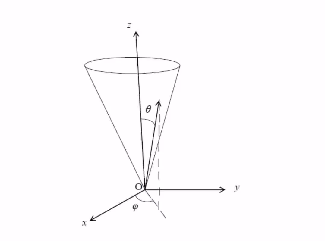
The unit for plane angle is radian (symbol = rad), while the unit for the solid angle is steradian (symbol = sr). Both of them are dimensionless quantities.

Whenever “mole” is used, the elementary entities in question (atoms, molecules, electrons, ions, etc.) must be clearly specified.

Derived physical quantities, such as speed, can be expressed in terms of fundamental physical quantities.

Measurement of length

A metre scale can be used to measure lengths from 10^-3 m to 10² m.

A Vernier callipers can be used for lengths to an accuracy of 10^-4 m.

A spherometer and a screw gauge can be used to measure lengths as small as 10^-5 m.

There are unique indirect methods for measuring lengths beyond the aforementioned ranges, which we will discuss below.

Measurement of large distances

You must certainly have realized that it is not possible to measure extremely large distances, such as the distance of a star or a planet from the earth, directly using a meter scale. In such situations, the parallax method is used for the measurement of the distance.

Hold up a pencil in front of your eyes against a fixed background, and look at it alternatively with each eye after closing the other eye. You will notice that the position of the pencil appears to change. This phenomenon is known as parallax.

The basis is defined as the distance between the two points of observation. In the above example, the basis corresponds to the distance between your eyes.

We can measure the distance D  of a planet P by observing it from two different positions A and B on the earth, separated by a distance AB = d. We can then measure the ∠APB, which is represented by the symbol θ and is known as the parallactic angle or the parallax angle.

Since the planet in question is at an extremely great distance, dD<<1. Thus, θ is very small. Therefore, we can approximately consider AB as an arc of length d of a circle with center at P, and the distance D as the radius AP=BP. Thus, AB=d=Dθ, where θ is in radians.

$$ D = \frac{b}{\theta}$$

Similarly, we can find out the size or angular diameter of the planet. If d is the diameter of the planet and α is the angular size of the planet (the angle subtended by d at the earth), then:

$$ \alpha = \frac{d}{D}$$

We can measure the angle α from the same place on the earth. Basically, it is the angle between two directions when we look at two diametrically opposite points on the planet using a telescope. We already know D, and can find out the diameter d using the equation given above.

Estimation of very small distances: the size of a molecule

We need to use special methods to measure very small distances, such as the size of a molecule (10^-8 to 10^-10 m). Obviously, we cannot use instruments like a meter scale or screw gauge, and even microscopes have certain limitations.

Let’s say you need to estimate the molecular size of oleic acid – a soapy liquid with large molecular size of the order of 10^-9 m. For this, you must begin by first creating a monomolecular layer of oleic acid on the surface of the water.

Dissolve 1 cm³ of oleic acid in alcohol and prepare a solution of 20 cm³. Take 1 cm³ of this solution and dilute it to 20 cm³ with the help of alcohol. Thus, the concentration of this solution will be equal to $\frac{1}{20 \times 20}$ cm³ of oleic acid/cm³ of solution.

Pour water in a large trough, sprinkle some lycopodium powder upon its surface and put one drop of the above solution on the surface. The drop will spread into a large and nearly circular film of molecular thickness on the water surface. Measure the diameter of this film to obtain its area A.

If you have dropped n drops in the water, you can find out the approximate volume of each drop (V cm³) as shown below:

Volume of n drops of solution = nV cm³

Amount of oleic acid in the solution = nV $\frac{1}{20 \times 20}$ cm³

Soon enough, the solution of oleic acid will spread further to form a very thin layer of thickness t. If it spreads to form a film of area A cm², then you can calculate t as shown below:

$$ t = \frac{Volume of the film}{Area of the film}$$

or $$ t = \frac{nV}{20×20A} cm$$

Assuming that this film has a monomolecular thickness, this becomes the size or diameter of a molecule of oleic acid. The value of this thickness is found to be of the order of 10^-9 m.

Range of lengths

The sizes of objects found in our universe are highly variable, ranging from the size of the order of 10^-14 m (the nucleus of an atom) to the size of the order of 10²⁶ m (the extent of the observable universe). You can see the range and order of sizes and lengths of some important objects below:

There are certain unique length units for exceptionally small and large lengths, which you can see below:

• 1 angstrom = 1 Å = 10^-10 m
• 1 fermi = 1 f = 10^-15 m
• 1 astronomical unit = 1 AU (average distance of the sun from the earth) = 1.496 × 10¹¹ m
• 1 lightyear = 1 ly = 9.46 × 10¹⁵ m (distance traveled by light in one year, with a velocity of 3 × 10⁸ m s^-1)
• 1 parsec = 3.08 × 10¹⁶ m (the distance at which the average radius of the earth’s orbit subtends an angle of 1 arc second)

Measurement of mass

Mass is a basic property of matter which is independent of the temperature, pressure, and location of the object in space.

The SI unit of mass is the kilogram (kg). However, it is an inconvenient unit when dealing with atoms and molecules. The unified atomic mass unit (u) is used in this case, which has been created to express the mass of atoms as follows:

1 unified atomic mass unit = 1 u = (1/12) of the mass of an atom of carbon-12 isotope (¹²C₆) including the mass of electrons = 1.66 × 10^-27 kg

A regular balance can be used to measure commonplace objects, whereas exceptionally large masses like stars and planets are measured by using the gravitational method, based on Newton’s law of gravitation.

The mass spectrograph is used to measure extremely small masses of atomic or subatomic particles. In this, the radius of the trajectory is proportional to the mass of a charged particle moving in a uniform electric and magnetic field.

Range of masses

Like length, the masses of objects encountered in the universe can be highly variable as well. They could range from the minuscule mass of an electron (of the order of 10^-30 kg) to the unimaginably large mass of the known universe (of the order of 10⁵⁵ kg).

Measurement of time

Today, we use an atomic standard if time which is based on the periodic vibrations produced in a caesium atom. This forms the basis of the caesium clock or atomic clock, which is used in national standards.

In the caesium atomic clock, a second is taken as the time required for 9,192,631,770 vibrations of the radiation corresponding to the transition between the two hyperfine levels of the ground state of the caesium-133 atom.

In India, a caesium clock is used at the National Physical Laboratory (NPL), New Delhi to maintain the Indian Standard Time (IST). These caesium atomic clocks are efficient enough to impart the uncertainty in time realisation as ± 1 × 10^-13.

By virtue of this great accuracy in the measurement of time, the SI unit of length has been expressed as the path length light travels in a certain interval of time (1/299,792,458 of a second).

Accuracy, the precision of instruments, and errors in measurement

There is a certain amount of uncertainty in the result of every measurement by any measuring instrument. There is an error in every calculated quantity based on measured values as well. In this regard, there are two important terms that one should know to differentiate between – accuracy and precision.

The accuracy of a measurement is a measure of how close the measured value is to the true value of the quantity. There could be various factors influencing the accuracy in measurement, including the resolution or the limit of the measuring instrument.

On the other hand, precision helps us understand the limit or resolution to which the quantity is measured.

The errors in measurement are broadly classified into two categories – systematic errors and random errors.

Systematic errors

These are errors that tend to be in one direction – either positive or negative. Given below are some of the sources of systematic errors:

• Instrumental errors that arise due to imperfect calibration or design of the measuring instrument, zero error in the instrument, and so on.
• Personal errors that arise due to bias or carelessness on the part of the person performing the experiment, or a lack of proper setting of the apparatus.
• Imperfection in experimental procedure or technique
• External conditions during the experiment, such as changes in humidity, temperature, wind velocity, and so on.

In order to minimize systematic errors, we need to remove personal bias, choose quality instruments, and improve experimental techniques as much as possible.

We can correctly estimate these errors for a given setup to some extent and apply the required corrections to the readings.

Random errors

These errors take place irregularly and are thus random with respect to size and sign. They can arise because of unpredictable and random changes in experimental conditions, personal (unbiased) errors by the observer taking readings, and so on.

For example, when the same person repeats the same observation, he could quite possibly get different readings every time.

Least count error

The least count of a measuring instrument is defined as the smallest value that can be measured by that particular instrument. For example, a spherometer could have a least count of 0.001 cm, while a Vernier’s caliper has a least count of 0.01 cm.

The error associated with the resolution of a measuring instrument is known as the least count error. It belongs to the category of random errors, but within a limited size; it can take place with both systematic and random errors.

The least count error can be reduced by improving experimental techniques, using instruments of higher precision, and so on.

We can ensure that the mean value is very close to the true value of the measured quantity by repeating the observations many times and taking the arithmetic mean of all the observations.

Absolute error, relative error and percentage error

Let us suppose that the various values obtained in a number of measurements are a₁, a₂, a₃, as so on… up to a_n. In this case, the arithmetic mean of these values is taken as the best possible value of the quantity under the given conditions of measurement, as given below:

$$ a_{mean} = \frac{a_1+a_2+\ldots+a_n}{n} $$

The magnitude of the difference between the individual measurement and the true value of the quantity is known as the absolute error of the measurement and is denoted by |∆a|.

The arithmetic mean is considered the true value if there is no other method of finding out the same. In that case, the errors in the individual measurement values from the true value are:

∆a₁ = a₁ – a_mean

∆a₂ = a₂ – a_mean

…

…

∆a_n = a_n – a_mean

Although the ∆a calculated above could be either positive or negative, the absolute error |∆a| is always positive.

The arithmetic mean of all the absolute errors is taken as the final or mean absolute error of the value of the physical quantity a, and is represented by ∆a_mean. Thus,

∆a_mean = (|∆a₁|+|∆a₂|+|∆a₃|+…+|∆a_n|) / n

The value we get upon doing a single measurement could be in the range a_mean ± ∆a_mean

i.e. a = a_mean ± ∆a_mean

or a_mean – ∆a_mean ≤ a ≤ a_mean + ∆a_mean

This means that any measurement of the physical quantity a could lie between (a_mean + ∆a_mean) and (a_mean – ∆a_mean).

The relative error or the percentage error (δa) is often used instead of the absolute error. It is defined as the ratio of the mean absolute error ∆a_mean to the mean value a_mean of the quantity measured.

Relative error = ∆a_mean / a_mean

The relative error is known as the percentage error (δa) when it is expressed in per cent.

This, percentage error δa = (∆a_mean / a_mean) × 100%

Combination of errors

Whenever you perform an experiment involving a lot of measurements, you must know how the errors in all the measurements combine in various mathematical operations. For example, we know that the density of a material is obtained by dividing its mass by its volume. If we have errors in the measurements of the mass and dimensions of the material, we must know what the error in its density will be.

Error of a sum or a difference

When two quantities are added or subtracted, the absolute error in the final result is the sum of the absolute errors in the individual quantities.

For example, let’s consider two physical quantities X and Y which have measured values X±∆X and Y±∆Y respectively, where ∆X and ∆Y are their absolute errors. We must now find the error ∆Z in the sum:

Z = X+Y

By addition, we have Z±∆Z = (X±∆X) + (Y±∆Y)

The maximum possible error in Z, ∆Z = ∆X+∆Y

Similarly, for the difference Z=A-B, we have:

Z±∆Z = (X±∆X) – (Y±∆Y)

          = (X-Y) ±∆X±∆Y

Or, ±∆Z = ±∆X±∆Y

In here, the maximum value of the error ∆Z is again ∆X+∆Y.

Error of a product or a quotient

When two quantities are multiplied or divided, the relative error in the result is the sum of the relative errors in the multipliers.

Once again, let’s consider two physical quantities X and Y which have measured values X±∆X and Y±∆Y respectively, and Z=XY. Then,

Z±∆Z = (X±∆X) (Y±∆Y) = XY±Y∆X±X∆Y±∆X∆Y

Dividing the LHS by Z and the RHS by XY, we get:

1±(∆Z/Z) = 1±(∆X/X) ±(∆Y/Y)±(∆X/X)(∆Y/Y)

∆X and ∆Y are extremely small, and therefore we can ignore their product. Thus, the maximum relative error will be:

∆Z/Z = (∆X/X) + (∆Y/Y)

It can be easily verified that this holds true for division as well.

Error in case of a measured quantity raised to a power

The relative error in a physical quantity raised to the power n is n times the relative error in the individual quantity.

Let’s say Z=X². In that case,

∆Z/Z = (∆X/X) + (∆X/X) = 2(∆X/X)

As you can see, the relative error in X² is two times the error in X.

Thus, we can say that if Z=A^pB^q/C^r, then:

∆Z/Z = p(∆A/A) + q(∆B/B) + r(∆C/C)

Significant figures

Since there are errors involved in every measurement, it is important to report the result of measurement in a way that indicates the precision of the instrument used.

Usually, the result of measurement is reported in the form of a number that, apart from all the digits in the number that are known reliably, also includes the first digit that is uncertain. The reliable digits plus the uncertain first digit are collectively known as significant figures or significant digits.

For example, the length of an object measured to be 395.6 cm has four significant figures – the digits 3, 9, and 5 are certain whereas the digit 6 is uncertain.

The number of significant figures or digits in a measurement is not affected by a choice of change of different units.

Given below are the important rules for determining the number of significant figures in a number:

• All the non-zero digits are significant.
• All the zeros between two non-zero digits are significant, regardless of where the decimal point is (if at all).
• For a number less than 1, the zero(s) on the right of the decimal point but to the left of the first non-zero digit are not significant.
• The trailing or terminal zero(s) in a number without a decimal point are not significant.
• The trailing zero(s) in a number with a decimal point are significant.
• For a number greater than 1 without any decimal, the trailing zero(s) are not significant.
• For a number with a decimal, the trailing zero(s) are significant.
• For measurements reported in scientific notation, the power of 10 is irrelevant to the determination of significant figures. However, the zeroes appearing in the base number in the scientific notation are significant.
• The digit 0 conventionally placed on the left of a decimal for a number less than 1 is not significant. However, the zeroes at the end of such a number are significant in a measurement.
• The multiplying and dividing factors that are neither rounded numbers nor numbers representing measured values are exact and have infinite number of significant digits.

Rules for arithmetic operations with significant figures

• During addition or subtraction, you should try to retain as many decimal places in the final result as there are in the original number with the least decimal places.
• During multiplication or division, you should try to retain as many significant figures in the final result as there are in the original number with the least significant figures.

Rounding off the uncertain digits

• If the insignificant digit to be dropped is more than 5, the preceding digit is raised by 1.
• If the insignificant digit to be dropped is less than 5, the preceding digit is not changed.
• If the preceding digit is even, the insignificant digit is simply dropped. If it is odd, the preceding digit is raised by 1.

Rules for determining the uncertainty in the results of arithmetic calculations

Let’s say the length and breadth of a thin rectangular sheet, measured using a meter scale, are 16.2 cm and 10.1 cm respectively. As you can see, there are three significant figures in each of these measurements.

The length l may be written as:

l = 16.2±0.1 cm = 16.2 cm±0.6%

Likewise, the breadth b may be written as b = 10.1±0.1 cm = 10.1 cm±1%

In this case, the error in the product of these values using the combination of errors rule wil be:

l b = 163.62 cm²±1.6% = 163.62±2.6 cm²

The final result will be: l b = 164±3 cm², where 3 cm² is the error or uncertainty in the estimation of area of rectangular sheet.

• In case a set of experimental data is specified to n significant figures, a result obtained by combining the data will also be valid to n significant figures.
• The relative error of a value of number specified to significant figures depends not only on n, but on the number itself as well.
• Intermediate results in a multistep computation need to be calculated to one more significant figure in every measurement than the number of digits in the least precise measurement.

Dimensions of physical quantities

All physical quantities represented by derived units can be expressed in terms of some combination of the seven base or fundamental units. These base quantities are known as the seven dimensions of the physical world, and are denoted with square brackets [ ], as shown below:

• Mass [M]
• Length [L]
• Time [T]
• Electric current [A]
• Thermodynamic temperature [K]
• Amount of substance [mol]
• Luminous intensity [cd]

The dimensions of a physical quantity are defined as the exponents or powers to which the base quantities are raised to represent that quantity.

For example, let’s consider a physical quantity like force. We know that the formula for force is as follows:

Force = mass × acceleration

           = mass × length / timetime

          = mass × length × (length)^-2

In the above example, you can see that the dimensions of force are 1 in mass, 1 in length, and -2 in time. Therefore,

[Force] = MLT^-2

Similarly, the dimensional formula for energy is given as follows:

[Energy] = ML²T^-2

This states that the dimensions of energy are 1 in mass, 2 in length, and -2 in time.

The expression which shows how and which of the base quantities represent the dimensions of a physical quantity is known as the dimensional formula of the given physical quantity.

An equation obtained by equating a physical quantity with its dimensional formula is called the dimensional equation of the physical quantity.

The principle of homogeneity

According to this principle, it is possible to multiply physical quantities with same or different dimensional formulae as required. However, only physical quantities with identical dimensional formulae can be added or subtracted. That is, if P+Q is valid, then both P and Q represent the same physical quantity.

Uses of dimensional analysis

There are several useful applications of dimensional analysis, which have been described below:

1. Converting units of a physical quantity from one system of units to another

This application is based on the following fact:

Numerical value × unit = constant

Thus, on changing the unit, the numerical value will get altered as well. Let’s suppose n₁ and n₂ are the numerical values of a given physical quantity, and u₁ and u₂ are the units in two different systems of units. Then,

n₁u₁ = n₂u₂

n₂ = n₁ M1 M2aL1 L2bT1 T2c

2. Checking the dimensional correctness of a given physical relation

This application is based on the principle of homogeneity, which states that a given physical relation is dimensionally correct if the dimensions of the different terms on either side of the relation are the same.

• sinθ, e^θ, cosθ, logθ give dimensionless values, and in the above expression θ is dimensionless 
• Powers are dimensionless.
• It is possible to add or subtract quantities having identical dimensions.

3. Establishing a relation between various physical quantities

If we know the different factors on which a physical quantity depends, then it is possible for us to find a relation among various factors by using the principle of homogeneity.

Limitations of dimensional analysis

• Dimensions are independent of the magnitude. Therefore, even the equation x = ut + at² is dimensionally correct. However, we know that this is not a physically correct equation. Thus, it is not necessary that a dimensionally correct equation is actually correct.
• Dimensional analysis is applicable only if the relation is of the product type. It cannot be used in the case of trigonometric and exponential relations.
• Numerical constants which are dimensionless cannot be deduced using dimensional analysis.
• This method does not distinguish between physical quantities having identical dimensions.

Calculating the order of magnitude

If the value of a physical quantity P satisfies the following condition:

0.5 × 10^x < P ≤ 5 × 10^x

Then x is an integer which is known as the order of magnitude.

For example, if the diameter of the sun is 13.9 × 10⁹ m, it can be expressed as 1.39 × 10¹⁰ m and the order of magnitude is 10.