The Prime Number Theorem and Open Frontiers - The Distribution of Primes Course

Statement and History

Theorem (Prime Number Theorem).

$$ \pi(x) \sim \frac{x}{\ln x} \quad \text{as } x \to \infty, $$

i.e., $ \lim_{x\to\infty} \pi(x)\ln(x)/x = 1 $.

History. Gauss conjectured this around 1792 based on numerical data. Legendre gave the approximation $ \pi(x) \approx x/(\ln x – 1.08366) $ in 1798. Chebyshev proved in 1852 that if the limit $ \pi(x)\ln(x)/x $ exists, it must equal 1; he also showed $ 0.92\ldots \leq \pi(x)\ln(x)/x \leq 1.10\ldots $ for all large $ x $.

The theorem was proved independently by Hadamard and de la Vallee Poussin in 1896, using Riemann’s idea of encoding prime distribution in the zeros of $ \zeta(s) $.

Prime counting function vs approximations

Distribution of prime gaps

Outline of the Analytic Proof

The proof has four key steps.

Step 1: Encode psi(x) via a Contour Integral (Perron’s Formula)

For $ c > 1 $ and $ x > 0 $,

$$ \psi(x) = \frac{1}{2\pi i}\int_{c-i\infty}^{c+i\infty} \left(-\frac{\zeta'(s)}{\zeta(s)}\right)\frac{x^s}{s}\,ds. $$

This follows from the Dirichlet series $ -\zeta'(s)/\zeta(s) = \sum_{n=1}^{\infty}\Lambda(n)n^{-s} $ and Mellin inversion (Perron’s formula).

Step 2: Show zeta(1 + it) is Never Zero

Theorem. $ \zeta(1 + it) \neq 0 $ for all real $ t \neq 0 $.

Proof. Use the trigonometric identity $ 3 + 4\cos\theta + \cos 2\theta \geq 0 $ (which follows from $ 3 + 4\cos\theta + \cos 2\theta = 2(1 + \cos\theta)^2 \geq 0 $). Taking logarithms of the Euler product:

$$ \ln|\zeta(\sigma + it)| = -\operatorname{Re}\sum_p\ln(1-p^{-\sigma-it}) = \sum_p\sum_{k=1}^{\infty}\frac{\cos(kt\ln p)}{kp^{k\sigma}}. $$

The identity gives

$$ 3\ln|\zeta(\sigma)| + 4\ln|\zeta(\sigma+it)| + \ln|\zeta(\sigma+2it)| \geq 0, $$

i.e., $ |\zeta(\sigma)|^3|\zeta(\sigma+it)|^4|\zeta(\sigma+2it)| \geq 1 $.

Near $ s=1 $, $ \zeta(\sigma) \sim 1/(\sigma-1) $, so if $ \zeta(1+it_0) = 0 $ then $ |\zeta(\sigma+it_0)|^4 = O((\sigma-1)^4) $ while $ |\zeta(\sigma)|^3 = O((\sigma-1)^{-3}) $. This forces $ |\zeta(\sigma+2it_0)| \geq c(\sigma-1)^{-1} \to \infty $, meaning $ \zeta $ has a pole at $ 1+2it_0 $. But $ \zeta $ is analytic at $ 1+2it_0 \neq 1 $, a contradiction.

This is one of the most elegant arguments in all of mathematics: a simple trigonometric inequality, combined with the Euler product, proves a deep fact about the zeros of the zeta function.

Step 3: Move the Contour

With $ \zeta(1+it) \neq 0 $ established, one shows there is a zero-free region of the form $ \operatorname{Re}(s) > 1 – c/\ln(|t|+2) $. Moving the contour in Perron’s formula leftward into this region picks up the residue at $ s=1 $ (giving $ x $) and a contour error term. The error term involves

$$ \frac{\zeta'(s)}{\zeta(s)} \ll \ln^2(|t|+2) $$

in the zero-free region, and careful estimation gives the error bound.

Step 4: Conclude

The calculation yields $ \psi(x) = x + O(x\exp(-c\sqrt{\ln x})) $, and partial summation converts this to the statement about $ \pi(x) $.

The Logarithmic Integral and Error Bounds

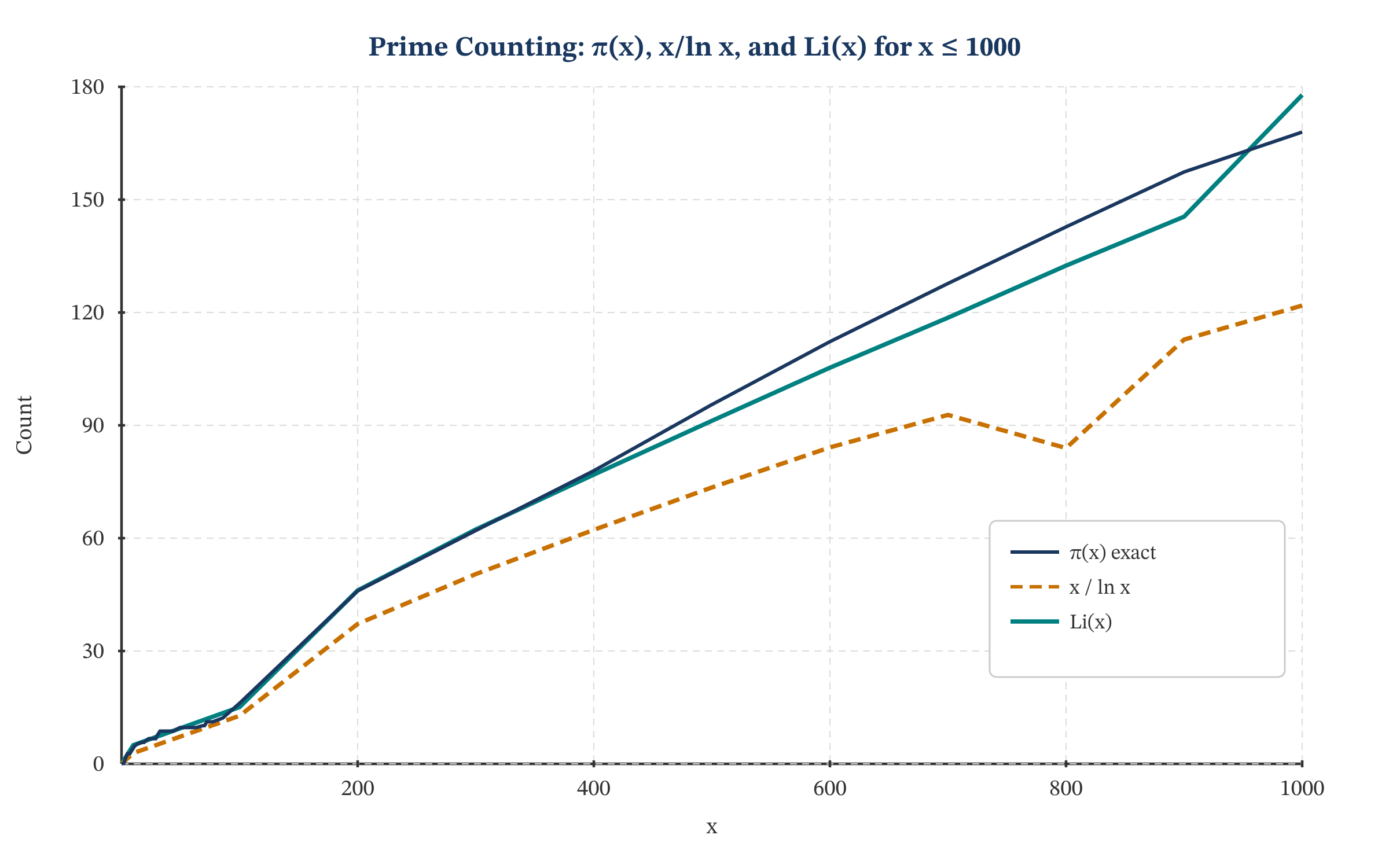
Definition. The offset logarithmic integral is

$$ \mathrm{Li}(x) = \int_2^x \frac{dt}{\ln t}. $$

Integration by parts gives $ \mathrm{Li}(x) = x/\ln x + x/\ln^2 x + 2x/\ln^3 x + \cdots $, so $ \mathrm{Li}(x)/(x/\ln x) \to 1 $ as $ x\to\infty $. The approximation $ \mathrm{Li}(x) $ is far more accurate than $ x/\ln x $:

$ x $: $ 10^3 $ | $ \pi(x) $: 168 | $ \lfloor x/\ln x \rfloor $: 144 | $ \lfloor\mathrm{Li}(x)\rfloor $: 177
$ x $: $ 10^4 $ | $ \pi(x) $: 1,229 | $ \lfloor x/\ln x \rfloor $: 1,085 | $ \lfloor\mathrm{Li}(x)\rfloor $: 1,245
$ x $: $ 10^6 $ | $ \pi(x) $: 78,498 | $ \lfloor x/\ln x \rfloor $: 72,382 | $ \lfloor\mathrm{Li}(x)\rfloor $: 78,627
$ x $: $ 10^8 $ | $ \pi(x) $: 5,761,455 | $ \lfloor x/\ln x \rfloor $: 5,428,681 | $ \lfloor\mathrm{Li}(x)\rfloor $: 5,762,208
$ x $: $ 10^{10} $ | $ \pi(x) $: 455,052,511 | $ \lfloor x/\ln x \rfloor $: 434,294,481 | $ \lfloor\mathrm{Li}(x)\rfloor $: 455,055,614$ \mathrm{Li}(x) $ consistently overestimates $ \pi(x) $ for $ x \leq 10^{23} $, but Littlewood proved in 1914 that $ \pi(x) – \mathrm{Li}(x) $ changes sign infinitely often. The first sign change (Skewes’ number) is known to occur before $ x \approx 1.4 \times 10^{316} $.

Theorem (de la Vallee Poussin, 1899).

$$ \pi(x) = \mathrm{Li}(x) + O\!\left(x\exp\!\bigl(-a\sqrt{\ln x}\,\bigr)\right) $$

for an explicit absolute constant $ a > 0 $.

Under RH the error is the much sharper $ O(\sqrt{x}\ln x) $.

Twin Primes: Bounded Gaps

Definition. Twin primes are pairs of primes of the form $ (p, p+2) $: $ (3,5), (5,7), (11,13), (17,19), \ldots $

Important: Twin Prime Conjecture. There are infinitely many twin prime pairs.

For decades, the best that could be proved was that the gap $ p_{n+1} – p_n $ is $ o(\ln p_n) $ infinitely often. In 2013, Zhang Yitang made a spectacular breakthrough:

Theorem (Zhang, 2013).

$$ \liminf_{n\to\infty}(p_{n+1} – p_n) \leq 70{,}000{,}000. $$

Zhang’s proof uses the Bombieri-Vinogradov theorem and an analysis of admissible tuples, building on the Goldston-Pintz-Yildirim (GPY) method.

Following Zhang’s announcement, the Polymath8 collaborative project rapidly reduced the bound. James Maynard (independently) introduced a new multidimensional sieve that dramatically simplified and improved the bound:

Theorem (Maynard, 2013; Polymath8b, 2014).

$$ \liminf_{n\to\infty}(p_{n+1} – p_n) \leq 246. $$

Under the Elliott-Halberstam conjecture, the bound reduces to 6. If the Elliott-Halberstam conjecture holds in a generalized form, the bound becomes 2, precisely the twin prime conjecture.

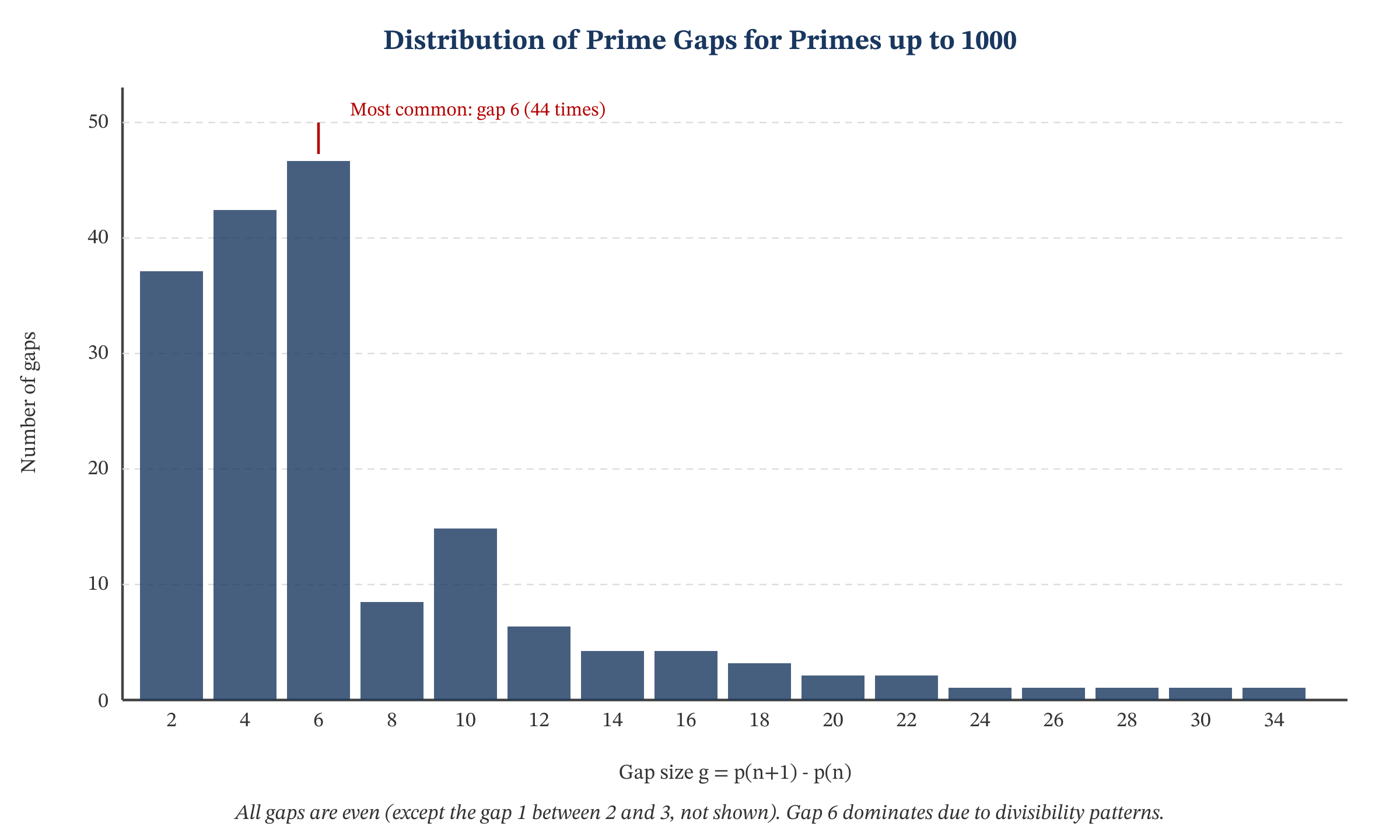
[Image: Gaps between consecutive primes for primes up to 500, showing preponderance of small gaps and occasional large ones]

Goldbach’s Conjecture

Important: Goldbach’s Conjecture (1742). Every even integer greater than 2 is the sum of two primes.

Verified for all even integers up to $ 4 \times 10^{18} $. The best partial results:

Vinogradov (1937): Every sufficiently large odd integer is the sum of three primes (using the circle method).
Helfgott (2013): Every odd integer $ \geq 7 $ is the sum of three primes (complete proof for the ternary Goldbach conjecture).
Chen (1973): Every large even integer is $ p + P_2 $ (prime plus semiprime).

The binary Goldbach conjecture remains open. A probabilistic heuristic (Hardy-Littlewood) predicts the number of representations of $ n $ as $ p + q $ to be asymptotically

$$ r_2(n) \sim 2\prod_{p>2}\frac{p-1}{p-2} \prod_{\substack{p\mid n\\p>2}}\frac{p-1}{p-2} \cdot\frac{n}{\ln^2 n}. $$

The Generalized Riemann Hypothesis

Definition. A Dirichlet L-function for a character $ \chi \pmod{q} $ is

$$ L(s, \chi) = \sum_{n=1}^{\infty}\frac{\chi(n)}{n^s} = \prod_p \frac{1}{1 – \chi(p)p^{-s}}, \quad \operatorname{Re}(s) > 1. $$

Important: Generalized Riemann Hypothesis (GRH).
All non-trivial zeros of $ L(s,\chi) $ for every primitive Dirichlet character $ \chi $ have real part $ 1/2 $.

GRH implies: the least prime in any arithmetic progression $ a, a+q, a+2q, \ldots $ (with $ \gcd(a,q)=1 $) is at most $ O(q^2\ln^2 q) $. It would also give a deterministic polynomial-time primality test.

Random Matrix Theory and the Zeros of Zeta

In 1972, Montgomery studied the pair correlation of zeros of $ \zeta(s) $. He found, and Freeman Dyson pointed out, that the pair correlation agrees with that of eigenvalues of random unitary matrices (GUE statistics):

Theorem (Montgomery, 1973, conditional on RH). Let $ \rho_n = 1/2 + i\gamma_n $ be the non-trivial zeros of $ \zeta(s) $. The normalized spacings have pair correlation function

$$ R_2(x) = 1 – \left(\frac{\sin(\pi x)}{\pi x}\right)^2, $$

the same as for eigenvalues of random Hermitian matrices.

This unexpected link has been confirmed numerically to extraordinary precision and drives an active research program. Katz and Sarnak extended these observations to families of $ L $-functions and related them to the classical compact groups $ U(N) $, $ SO(2N) $, $ USp(2N) $.

Primes in Short Intervals and Cramer’s Model

Cramer’s probabilistic model treats $ \mathbf{1}_{n \text{ is prime}} $ as independent Bernoulli variables with probability $ 1/\ln n $. Under this model:

Maximal prime gap up to $ x $: $ \sim \ln^2 x $ (Cramer’s conjecture).
Every interval $ (x, x + C\ln^2 x) $ contains a prime for large $ x $.

Conditionally on RH, the best proved result is that $ (x, x + x^{1/2+\varepsilon}) $ contains a prime for any $ \varepsilon > 0 $ and large $ x $. Unconditionally, Baker-Harman-Pintz (2001) gives the exponent $ 0.525 $.

The Bombieri-Vinogradov Theorem

Theorem (Bombieri-Vinogradov, 1965). For any $ A > 0 $ there exists $ B = B(A) $ such that

$$ \sum_{q \leq \sqrt{x}/\ln^B x} \max_{y \leq x}\max_{\gcd(a,q)=1} \left|\psi(y;q,a) – \frac{y}{\phi(q)}\right| \ll \frac{x}{\ln^A x}, $$

where $ \psi(x; q, a) = \sum_{n \leq x,\,n \equiv a \pmod{q}} \Lambda(n) $.

This says primes are, on average over moduli $ q \leq \sqrt{x}/\ln^B x $, as well distributed as GRH would predict, sometimes called a “poor man’s GRH.”

The Millennium Prize Problem

In May 2000, the Clay Mathematics Institute announced seven Millennium Prize Problems, each carrying a $1,000,000 prize. The Riemann Hypothesis is number 8 on Hilbert’s 1900 list and one of the seven Millennium Problems.

What a proof (or disproof) would accomplish:

A proof would immediately give the sharp error term $ \pi(x) = \mathrm{Li}(x) + O(\sqrt{x}\ln x) $, settling a century of work on the distribution of primes.
It would prove dozens of theorems currently stated “conditionally on RH”: explicit bounds in Dirichlet’s theorem and results throughout algebraic number theory.
A disproof would be equally revolutionary: a zero off the critical line would force a rethink of the heuristics of prime distribution and the random matrix connection.
The method of proof or disproof would almost certainly open entirely new chapters of mathematics.

Progress towards a proof has come from many directions: zero-free regions (Vinogradov-Korobov, 1958), density theorems (bounding the number of zeros with $ \operatorname{Re}(s) > \sigma $ for $ \sigma > 1/2 $), $ p $-adic methods, and spectral interpretations (Connes’ noncommutative geometry, Deninger’s programme). None has yet succeeded.

The Elementary Proof

In 1949, Erdos and Selberg independently found an “elementary” proof of the PNT, one that avoids complex analysis entirely. The key ingredient is Selberg’s asymptotic formula:

$$ \sum_{p \leq x} \ln^2 p + \sum_{pq \leq x} \ln p \cdot \ln q = 2x\ln x + O(x). $$

This identity, proved using only real-variable methods and the Mobius function, encodes enough information about the distribution of primes to force $ \psi(x) \sim x $. The proof proceeds by showing that if $ \psi(x)/x $ deviates from 1, the Selberg formula leads to a contradiction.

The elementary proof was historically significant but is not “simpler” than the analytic proof. It merely avoids complex analysis, replacing it with intricate combinatorial estimates. Most modern treatments of the PNT use the analytic approach, which provides sharper error terms.

The Riemann-von Mangoldt Formula

Let $ N(T) = |\{\rho : \zeta(\rho) = 0,\, 0 < \operatorname{Re}(\rho) < 1,\, 0 < \operatorname{Im}(\rho) \leq T\}| $. Then

$$ N(T) = \frac{T}{2\pi}\ln\frac{T}{2\pi e} + \frac{7}{8} + O(\ln T). $$

So zeros become increasingly dense at height $ T $, with average spacing $ \sim 2\pi/\ln T $.

Exercises:

Using the table of $ \pi(x) $ values, compute $ \pi(10^6) \cdot \ln(10^6) / 10^6 $ and verify it is close to 1 (as predicted by PNT).

Compute $ \mathrm{Li}(100) = \int_2^{100} dt/\ln t $ numerically (use a calculator or Riemann sums) and compare with $ \pi(100) = 25 $.

The “3-4-1” inequality $ 3 + 4\cos\theta + \cos 2\theta \geq 0 $ is used to prove $ \zeta(1+it) \neq 0 $. Verify this inequality by expanding $ \cos 2\theta = 2\cos^2\theta – 1 $ and showing the result equals $ 2(1 + \cos\theta)^2 $.

List all twin prime pairs $ (p, p+2) $ with $ p < 200 $. How does the count compare with $ C \cdot 200/\ln^2(200) $ for $ C \approx 1.32 $ (the twin prime constant)?

Verify Goldbach’s conjecture for every even integer from 4 to 50 by exhibiting at least one representation as a sum of two primes.

If the Riemann Hypothesis is true, the error in the PNT is $ O(\sqrt{x}\ln x) $. For $ x = 10^{10} $, estimate $ \sqrt{x}\ln x $ and compare it with the actual error $ |\pi(10^{10}) – \mathrm{Li}(10^{10})| \approx 3{,}103 $.

The Riemann-von Mangoldt formula gives $ N(T) \approx (T/2\pi)\ln(T/2\pi e) $. Estimate how many non-trivial zeros have imaginary part less than 100.