The Circle Method and Exact Formulas - Ramanujan's Partition Function Course

How fast does $ p(n) $ grow? In 1918, Hardy and Ramanujan answered this question with one of the most powerful techniques in analytic number theory: the circle method. In 1937, Rademacher refined their approach into an exact convergent formula. This lesson traces the path from the Cauchy integral through Farey fractions and Ford circles to Rademacher’s exact formula, and then explores the Rogers-Ramanujan identities and mock theta functions.

The circle method in the complex plane

Ford circles and the circle method

Growth of p(n)

Before the Hardy-Ramanujan work of 1918, the only known asymptotic result for $ p(n) $ was the empirical observation that $ p(n) $ grows faster than any polynomial. The precise asymptotic was established by Hardy and Ramanujan:

Theorem (Hardy-Ramanujan, 1918). As $ n \to \infty $:

$$ p(n) \sim \frac{1}{4n\sqrt{3}}\,\exp\!\left(\pi\sqrt{\frac{2n}{3}}\right). $$

For $ n = 200 $ this gives $ p(200) \approx 4.10 \times 10^{12} $, compared to the exact value $ p(200) = 3{,}972{,}999{,}029{,}388 $. The relative error is less than 3.5%.

$ n $: 10 | $ p(n) $ (exact): 42 | HR formula: 48.1 | Relative error: 14.5%
$ n $: 20 | $ p(n) $ (exact): 627 | HR formula: 686 | Relative error: 9.4%
$ n $: 50 | $ p(n) $ (exact): 204,226 | HR formula: 217,000 | Relative error: 6.3%
$ n $: 100 | $ p(n) $ (exact): 190,569,292 | HR formula: 199,280,893 | Relative error: 4.6%
$ n $: 200 | $ p(n) $ (exact): 3,972,999,029,388 | HR formula: 4,100,251,432,188 | Relative error: 3.2%
The relative error decreases as $ n $ grows, consistent with the formula being asymptotic rather than exact.

Setting Up the Cauchy Integral

The generating function $ F(q) = \sum_{n \geq 0} p(n) q^n $ converges for $ |q| < 1 $. By Cauchy’s integral formula,

$$ p(n) = \frac{1}{2\pi i}\oint_{|q|=r} \frac{F(q)}{q^{n+1}}\,dq, $$

for any $ 0 < r < 1 $. Write $ q = e^{2\pi i \tau} $ with $ \tau = x + iy $, $ y > 0 $. The substitution $ r = e^{-2\pi y} $ transforms this into an integral over the unit interval in $ x $:

$$ p(n) = \int_0^1 F(e^{2\pi i(x+iy)})\,e^{-2\pi i n(x+iy)}\,dx. $$

The integrand is largest near $ x = 0 $ because $ F(q) \to \infty $ as $ \tau \to 0 $ (i.e., $ q \to 1 $).

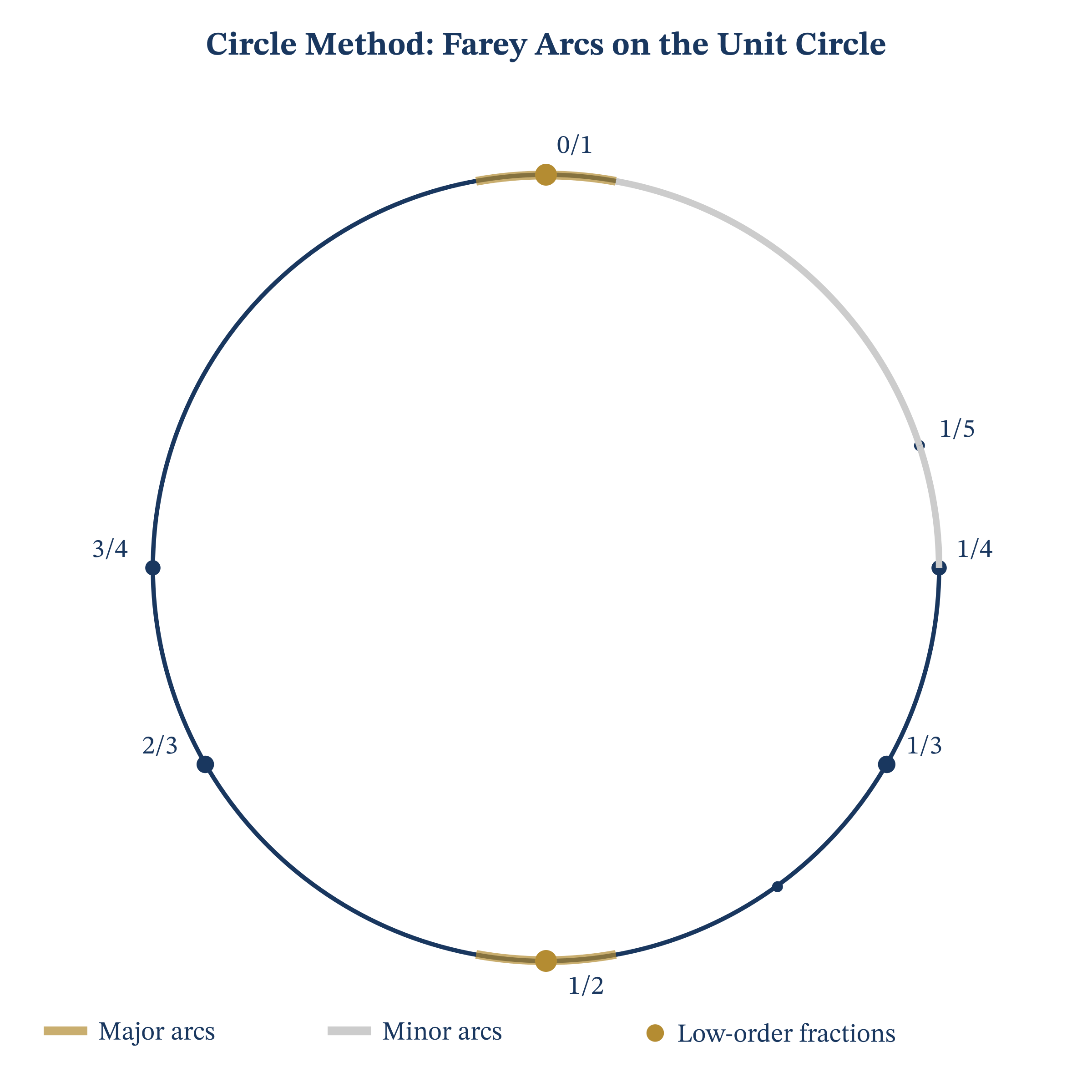
Farey Fractions and the Farey Dissection

The Farey sequence $ \mathcal{F}_N $ is the sequence of reduced fractions $ h/k $ with $ 0 \leq h/k \leq 1 $ and $ 1 \leq k \leq N $, arranged in increasing order.

For $ N = 4 $: $ \mathcal{F}_4 = \{0/1,\; 1/4,\; 1/3,\; 1/2,\; 2/3,\; 3/4,\; 1/1\} $.

[Image: The Farey dissection of the unit interval, with integration contour divided into arcs centered on Farey fractions]

The key property of Farey sequences is:

Lemma (Farey Neighbours). If $ h/k $ and $ h’/k’ $ are adjacent in $ \mathcal{F}_N $, then $ |hk’ – h’k| = 1 $ and $ k + k’ \geq N + 1 $.

The Farey dissection partitions the interval $ [0,1] $ into arcs $ I_{h,k} $ centered at each $ h/k \in \mathcal{F}_N $. On the arc $ I_{h,k} $, the generating function $ F(e^{2\pi i\tau}) $ behaves predictably via the modular transformation properties of the eta function.

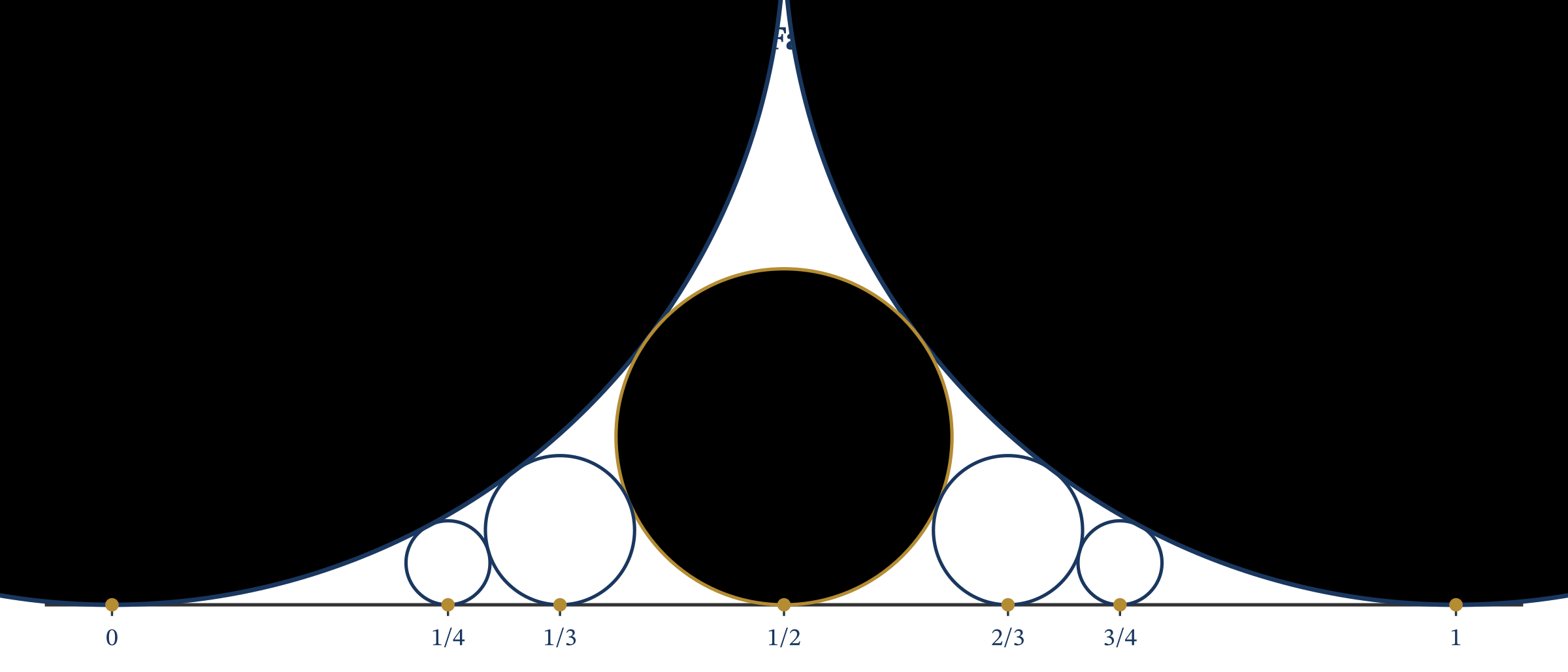
Ford Circles

The Ford circle $ C(h,k) $ for a reduced fraction $ h/k $ is the circle of radius $ 1/(2k^2) $ tangent to the real axis at $ h/k $.

[Image: Ford circles for the Farey fractions of order 5, showing tangency between adjacent circles]

Lemma. Two Ford circles $ C(h,k) $ and $ C(h’,k’) $ are either externally tangent or disjoint. They are tangent if and only if $ h/k $ and $ h’/k’ $ are adjacent in some Farey sequence, equivalently $ |hk’ – h’k| = 1 $.

Proof. The centers of $ C(h,k) $ and $ C(h’,k’) $ are $ (h/k, 1/(2k^2)) $ and $ (h’/k’, 1/(2k’^2)) $. The squared distance between the centers is

$$ \left(\frac{h}{k} – \frac{h'}{k'}\right)^2 + \left(\frac{1}{2k^2} – \frac{1}{2k'^2}\right)^2 = \frac{(hk'-h'k)^2}{k^2 k'^2} + \frac{(k'^2-k^2)^2}{4k^4 k'^4}. $$

The sum of radii is $ \frac{1}{2k^2} + \frac{1}{2k’^2} $. The circles are tangent when the distance between centers equals the sum of radii, which occurs precisely when $ |hk’ – h’k| = 1 $. $ \blacksquare $

Modular Transformation of the Eta Function

The key analytic input is the transformation formula for the Dedekind eta function $ \eta(\tau) = e^{\pi i\tau/12}\prod_{n=1}^{\infty}(1-e^{2\pi i n\tau}) $.

Theorem (Modular Transformation). For $ \operatorname{Im}(\tau) > 0 $ and $ \begin{pmatrix}a&b\\c&d\end{pmatrix} \in \mathrm{SL}_2(\mathbb{Z}) $ with $ c > 0 $:

$$ \eta\!\left(\frac{a\tau+b}{c\tau+d}\right) = \epsilon(a,b,c,d)\,(-i)^{1/2}(c\tau+d)^{1/2}\,\eta(\tau), $$

where $ \epsilon(a,b,c,d) $ is a certain 24th root of unity related to Dedekind sums.

Applied to the arc near $ h/k \in \mathcal{F}_N $, with $ \tau = h/k + iz/(k^2) $ for small $ z $, the generating function satisfies

$$ F(e^{2\pi i\tau}) \sim \exp\!\left(\frac{\pi^2}{6k^2 z} + \frac{\pi z}{6}\right) \cdot (\text{exponentially smaller corrections}), $$

and the main contribution to the Cauchy integral comes from the arc near $ h/k = 0/1 $ (i.e., $ k=1 $).

Derivation of the Asymptotic

The Saddle-Point Method

The dominant contribution to the Cauchy integral comes from a neighborhood of $ q = 1 $. Writing $ q = e^{-w} $ with $ w = \epsilon – 2\pi i\theta $ for small $ \epsilon > 0 $:

$$ p(n) = \int_{-1/2}^{1/2} F(e^{-\epsilon+2\pi i\theta})\,e^{n(\epsilon-2\pi i\theta)}\,d\theta. $$

As $ \epsilon \to 0^+ $, the generating function behaves near $ \theta = 0 $ via the modular transformation:

$$ \log F(e^{-w}) = \frac{\pi^2}{6w} – \frac{1}{2}\log w + \frac{1}{2}\log(2\pi) + O(e^{-2\pi^2/w}). $$

Setting $ w = 2\pi(\epsilon – 2\pi i\theta) $ and optimizing over $ \epsilon $ via the saddle point condition, one finds the optimal radius

$$ \epsilon^* = \frac{\pi}{\sqrt{6n}}, $$

giving the leading exponential $ e^{\pi\sqrt{2n/3}} $.

The Gaussian integral around the saddle point:

$$ \int_{-\infty}^{\infty} e^{-2\pi^2 n\theta^2/\epsilon^*}\,d\theta = \sqrt{\frac{\epsilon^*}{2\pi^2 n}}, $$

which, combined with the prefactor, gives the Hardy-Ramanujan formula.

Contributions from All Arcs

Hardy and Ramanujan showed that the contributions from all arcs $ I_{h,k} $ with $ k \leq N $ give:

$$ p(n) = \sum_{k=1}^{N} \Phi_{h,k}(n) + O(n^{-1/4}), $$

where $ \Phi_{h,k}(n) $ is the contribution from the arc near $ h/k $, and the dominant term is

$$ \Phi_{0,1}(n) = \frac{\sqrt{3}}{2\pi\sqrt{2}}\,n^{-3/4}\,\left(1 – \frac{\sqrt{3}}{4\pi\sqrt{2n}}\right)\,e^{\pi\sqrt{2n/3}}. $$

For large $ n $, all other arcs contribute terms of smaller exponential order.

Rademacher’s Exact Formula

Hardy and Ramanujan’s formula is asymptotic: the error term $ O(n^{-1/4}) $ does not vanish. In 1937, Hans Rademacher showed how to convert the method into an exact convergent formula by summing over all Farey fractions.

Theorem (Rademacher’s Exact Formula, 1937). For all $ n \geq 1 $:

$$ p(n) = \frac{1}{\pi\sqrt{2}}\sum_{k=1}^{\infty} A_k(n)\,\sqrt{k}\,\frac{d}{dn} \left[\frac{\sinh\!\left(\frac{\pi}{k}\sqrt{\frac{2}{3}\left(n-\frac{1}{24}\right)}\right)} {\sqrt{n – \frac{1}{24}}}\right], $$

where $ A_k(n) = \sum_{\substack{0 \leq h < k \\ \gcd(h,k)=1}} e^{\pi i s(h,k) – 2\pi i n h/k} $ and $ s(h,k) $ is the Dedekind sum.

The series on the right converges to the exact integer value of $ p(n) $, so one can compute $ p(n) $ by taking enough terms and rounding.

Kloosterman Sums and Dedekind Sums

The sums $ A_k(n) $ are a special case of Kloosterman sums. For integers $ m $, $ n $, $ k $ with $ k \geq 1 $:

$$ \mathrm{Kl}(m, n; k) = \sum_{\substack{a=1\\\gcd(a,k)=1}}^{k} e^{2\pi i(ma + n\bar{a})/k}, $$

where $ \bar{a} $ is the multiplicative inverse of $ a $ modulo $ k $. Kloosterman sums satisfy the Weil bound $ |\mathrm{Kl}(m,n;k)| \leq d(k)\sqrt{k} $, proved using the Riemann Hypothesis for curves over finite fields.

The Dedekind sum is

$$ s(h, k) = \sum_{j=1}^{k-1}\left(\!\left(\frac{j}{k}\right)\!\right) \left(\!\left(\frac{hj}{k}\right)\!\right), $$

where $ ((x)) = x – \lfloor x \rfloor – 1/2 $ if $ x \notin \mathbb{Z} $, and 0 if $ x \in \mathbb{Z} $.

Dedekind sums satisfy the reciprocity law:

$$ s(h, k) + s(k, h) = \frac{h}{12k} + \frac{k}{12h} + \frac{1}{12hk} – \frac{1}{4}, $$

a formula analogous to the law of quadratic reciprocity.

Convergence

The series converges absolutely for every $ n \geq 1 $. Using the bound $ |A_k(n)| \leq k $, the $ k $-th term is bounded by

$$ O\!\left(k^{3/2}\,e^{\pi\sqrt{2n/3}/k}\right), $$

and since $ \sum_{k=1}^{\infty} k^{3/2}e^{-ck} $ converges for any $ c > 0 $, the series converges absolutely as soon as $ n \geq 1 $.

Computing p(n) Exactly

Taking the first few terms of Rademacher’s series already gives a startlingly accurate approximation.

For $ p(100) = 190{,}569{,}292 $, using $ K = 5 $ terms:

$ k $: 1 | Contribution: 190,568,944.37…
$ k $: 2 | Contribution: 355.13…
$ k $: 3 | Contribution: -1.97…
$ k $: 4 | Contribution: 0.47…
$ k $: 5 | Contribution: -0.07…
Sum: $ 190{,}569{,}298.\ldots $ Rounding to the nearest integer: $ 190{,}569{,}292 $. The number of terms required to achieve rounding accuracy grows like $ O(\sqrt{n}) $.

Bessel Function Form

The exact formula can be rewritten using the modified Bessel function. Define $ \lambda_k(n) = \pi\sqrt{\frac{2}{3}(n – \frac{1}{24})}\cdot\frac{1}{k} $. Then:

$$ p(n) = \frac{2\pi}{(24n-1)^{3/4}} \sum_{k=1}^{\infty} A_k(n)\,k^{-1/2}\,I_{3/2}(\lambda_k(n)), $$

where $ I_{3/2} $ is the modified Bessel function of the first kind.

The Rogers-Ramanujan Identities

Among the most celebrated identities in all of combinatorics:

Theorem (Rogers-Ramanujan Identities). For $ |q| < 1 $:

$$ \sum_{n=0}^{\infty}\frac{q^{n^2}}{(1-q)(1-q^2)\cdots(1-q^n)} = \prod_{n=1}^{\infty}\frac{1}{(1-q^{5n-1})(1-q^{5n-4})}, $$ $$ \sum_{n=0}^{\infty}\frac{q^{n^2+n}}{(1-q)(1-q^2)\cdots(1-q^n)} = \prod_{n=1}^{\infty}\frac{1}{(1-q^{5n-2})(1-q^{5n-3})}. $$

Important: The left side of the first identity counts partitions of $ n $ where consecutive parts differ by at least 2. The right side counts partitions of $ n $ into parts $ \equiv \pm 1 \pmod{5} $. These two families have the same count for every $ n $, a highly non-obvious bijection. Similarly for the second identity: parts differing by at least 2 with smallest part at least 2, versus parts $ \equiv \pm 2 \pmod{5} $.

These identities were discovered by Rogers (1894), rediscovered by Ramanujan (c. 1913), and proved jointly in 1919. A deep approach shows the identities follow from the representation theory of the affine Lie algebra $ A_1^{(1)} $.

The Jacobi Triple Product Identity

Theorem. For $ |q| < 1 $ and $ z \neq 0 $:

$$ \sum_{n=-\infty}^{\infty} z^n q^{n^2} = \prod_{n=1}^{\infty}(1-q^{2n})(1+zq^{2n-1})(1+z^{-1}q^{2n-1}). $$

Setting $ z = q $ and replacing $ q $ by $ q^{1/2} $ recovers Euler’s pentagonal number theorem. Setting $ z = q^2 $ and replacing $ q $ by $ q^{1/2} $ gives Jacobi’s four-square theorem: every positive integer can be expressed as a sum of four squares in exactly $ r_4(n) = 8\sum_{4 \nmid d \mid n} d $ ways.

Bailey’s Lemma and q-Series

The Rogers-Ramanujan identities fit into the framework of Bailey pairs. A Bailey pair relative to $ a $ is a pair of sequences $ (\alpha_n, \beta_n)_{n \geq 0} $ satisfying

$$ \beta_n = \sum_{r=0}^{n}\frac{\alpha_r}{(q;q)_{n-r}(aq;q)_{n+r}}, $$

where $ (a;q)_n = \prod_{j=0}^{n-1}(1-aq^j) $.

Bailey’s lemma generates an infinite “Bailey chain” of identities from a single Bailey pair, each as beautiful as the Rogers-Ramanujan originals.

Mock Theta Functions

Near the end of his life, Ramanujan introduced a set of $ q $-series he called mock theta functions. A typical example is:

$$ f(q) = \sum_{n=0}^{\infty}\frac{q^{n^2}}{(1+q)^2(1+q^2)^2\cdots(1+q^n)^2}. $$

Ramanujan observed that these functions, like theta functions, have modular-transformation-like properties, but they are not genuine modular forms.

The theoretical explanation came in 2002 when Zwegers showed that mock theta functions are the “holomorphic parts” of certain harmonic Maass forms: real-analytic modular forms that satisfy the Laplacian equation but are not holomorphic. This discovery opened a new field and led directly to the Bruinier-Ono formula.

Modern Developments

Modular Forms and the Partition Function

The generating function for $ p(n) $, written in terms of $ \tau \in \mathbb{C} $ with $ \operatorname{Im}(\tau) > 0 $ and $ q = e^{2\pi i\tau} $, is:

$$ \sum_{n=0}^{\infty} p(n)\,q^{n-1/24} = \frac{1}{\eta(\tau)}, $$

where $ \eta(\tau) = q^{1/24}\prod_{n=1}^{\infty}(1-q^n) $ is the Dedekind eta function. The function $ 1/\eta(\tau) $ is a modular form of weight $ -1/2 $ for $ \Gamma_0(576) $ with a suitable multiplier system.

The Bruinier-Ono Algebraic Formula

In 2011, Bruinier and Ono found a completely different formula for $ p(n) $ expressed as a finite sum of algebraic numbers.

Theorem (Bruinier-Ono, 2011). For $ n \geq 1 $, let $ \Delta = 1 – 24n $ and let $ H(\Delta) $ be the ring class field of $ \mathbb{Q}(\sqrt{\Delta}) $. There exist explicit algebraic integers $ \alpha_Q(n) \in H(\Delta) $ indexed by certain quadratic forms $ Q $ of discriminant $ \Delta $ such that

$$ p(n) = \frac{1}{24n – 1}\sum_Q \alpha_Q(n), $$

where the sum is finite.

This formula is of a fundamentally different character from Rademacher’s: Rademacher’s formula converges from an infinite series involving transcendental quantities (hyperbolic sines), while Bruinier and Ono’s formula is an exact finite sum of algebraic numbers.

Connections to Physics

Partitions appear throughout theoretical physics:

Statistical mechanics. The number of ways of distributing $ n $ bosonic quanta among energy levels corresponds to the number of partitions. The Hardy-Ramanujan formula gives the density of states.
String theory. The Hagedorn temperature, at which string partition functions diverge, is governed by the exponential growth of $ p(n) $.
Black hole entropy (the Cardy formula). In $ \mathrm{AdS}_3/\mathrm{CFT}_2 $ duality, the entropy of BTZ black holes is given by

$$ S \sim 2\pi\sqrt{\frac{cn}{6}}, $$

where $ c $ is the central charge of the dual CFT. This is essentially the Hardy-Ramanujan asymptotic.

Topological string theory. The generating function $ \prod(1-q^n)^{-1} $ and its relatives appear as partition functions of topological quantum field theories. Plane partitions count degeneracies of BPS states in type-IIA string theory.

Open Problems

Effective Rademacher formula. How many terms of Rademacher’s series are needed to determine $ p(n) $ exactly? The answer is conjectured to be $ O(\sqrt{n}) $ but not proved in full generality.
New congruences. While Ono proved infinitely many congruences exist for each prime $ \ell \geq 5 $, finding them explicitly for large $ \ell $ remains a challenge.
Plane and solid partitions. MacMahon’s generating function for plane partitions is $ \prod_{n=1}^{\infty}(1-q^n)^{-n} $. The asymptotic and exact formulas for plane partition counts are significantly harder.
Algebraic structure of $ p(n) $. The Bruinier-Ono formula raises the question: what algebraic number fields arise? Are there patterns in the Galois-theoretic properties of the algebraic integers $ \alpha_Q(n) $?

Exercises

Compute the Farey sequence $ \mathcal{F}_5 $ and verify the property that for each pair of adjacent fractions $ h/k $ and $ h’/k’ $, we have $ |hk’ – h’k| = 1 $.
Draw the Ford circles for $ \mathcal{F}_3 $ and verify that adjacent Farey fractions produce tangent circles.
Using the leading term of Rademacher’s formula (the $ k = 1 $ term), estimate $ p(50) $ and compare with the exact value 204,226.
Verify the first Rogers-Ramanujan identity for $ n = 7 $: list all partitions of 7 into parts differing by at least 2, and all partitions of 7 into parts $ \equiv \pm 1 \pmod{5} $.
Compute the Dedekind sum $ s(1, 5) $ directly from the definition.
The mock theta function $ f(q) = \sum_{n=0}^{\infty} q^{n^2}/\prod_{j=1}^{n}(1+q^j)^2 $. Compute the first 5 nonzero coefficients of this power series.
The Cardy formula $ S \sim 2\pi\sqrt{cn/6} $ matches the Hardy-Ramanujan exponent $ \pi\sqrt{2n/3} $ when $ c = 1 $. If the central charge is $ c = 24 $ (as in the Monster module), what is the asymptotic growth exponent?