Ramanujan, Ford Circles, and the Stern-Brocot Tree

Continued fractions connect to some of the deepest and most visually stunning objects in mathematics. In this lesson we explore three remarkable topics: Ramanujan’s continued fraction identities, the geometric world of Ford circles and Farey sequences, and the Stern-Brocot tree, a structure that organizes every positive rational number into a single binary tree.

Ford circles and the Farey sequence

The Stern-Brocot tree

Generalized Continued Fractions

Definition. A generalized continued fraction has the form

$$ b_0 + \dfrac{a_1}{\displaystyle b_1 + \dfrac{a_2}{\displaystyle b_2 + \dfrac{a_3}{\displaystyle b_3 + \ddots}}} $$

where the $ a_i $ and $ b_i $ need not be positive integers.

Euler’s Continued Fraction for $ e $

Important: The base of the natural logarithm has the simple continued fraction expansion
$$ > e = [2; 1, 2, 1, 1, 4, 1, 1, 6, 1, 1, 8, 1, 1, 10, \ldots] > $$
with the remarkable pattern: the partial quotients follow the repeating pattern $ 1, 2k, 1 $ as $ k $ runs through $ 1, 2, 3, \ldots $

This follows from Euler’s generalized CF for $ (e^{x/y} – 1)/(e^{x/y} + 1) $:

$$ \frac{e^{x/y} – 1}{e^{x/y} + 1} = \dfrac{x}{\displaystyle 2y + \dfrac{x^2}{\displaystyle 6y + \dfrac{x^2}{\displaystyle 10y + \dfrac{x^2}{\displaystyle 14y + \ddots}}}} $$

Setting $ x = y = 1 $ and manipulating gives the pattern for $ e $.

The first several convergents of $ e $ are:

$$ 2,\; 3,\; \frac{8}{3},\; \frac{11}{4},\; \frac{19}{7},\; \frac{87}{32},\; \frac{106}{39},\; \frac{193}{71},\; \frac{1264}{465},\; \frac{1457}{536},\; \ldots $$

The convergent $ 193/71 = 2.71830\ldots $ approximates $ e = 2.71828\ldots $ to nearly 5 decimal places. The convergents just before the large partial quotients (the $ 2k $ terms) give especially good approximations.

Irrationality of $ e $. Since $ e = [2; 1, 2, 1, 1, 4, 1, 1, 6, \ldots] $ is an infinite CF (the partial quotients $ 2k $ grow without bound), $ e $ is irrational. Moreover, since the partial quotients are unbounded, $ e $ is not a quadratic irrational (by Lagrange’s theorem, quadratic irrationals have eventually periodic, hence bounded, CFs). Hermite proved in 1873 that $ e $ is transcendental, a far stronger result.

Tip: Euler also discovered that $ \sqrt{e} = [1; 1, 1, 1, 5, 1, 1, 9, 1, 1, 13, 1, 1, 17, \ldots] $ with pattern $ \sqrt{e} = [1; \overline{1, 1, 4k+1}]_{k=0}^{\infty} $.

Lambert’s Proof of the Irrationality of $ \pi $

The tangent function has the generalized continued fraction:

$$ \tan x = \dfrac{x}{\displaystyle 1 – \dfrac{x^2}{\displaystyle 3 – \dfrac{x^2}{\displaystyle 5 – \dfrac{x^2}{\displaystyle 7 – \ddots}}}} $$

Theorem (Lambert, 1761). $ \pi $ is irrational.

Proof sketch. Lambert showed that if $ x \neq 0 $ is rational, then the CF for $ \tan x $ converges to an irrational value. For $ x = p/q $, the CF becomes

$$ \tan(p/q) = \dfrac{p}{\displaystyle q – \dfrac{p^2}{\displaystyle 3q – \dfrac{p^2}{\displaystyle 5q – \ddots}}} $$

The denominators $ (2n+1)q $ eventually exceed $ p^2 + 1 $, satisfying an irrationality criterion for generalized CFs. Since $ \tan(\pi/4) = 1 $ is rational, $ \pi/4 $ must be irrational, hence $ \pi $ is irrational. $ \square $

The hyperbolic tangent has a parallel CF (with plus signs instead of minus), and replacing $ x $ by $ ix $ recovers Lambert’s formula, connecting the circular and hyperbolic functions through continued fractions.

Ramanujan’s Continued Fractions

Ramanujan discovered many spectacular continued fraction identities.

The Rogers-Ramanujan Continued Fraction

For $ |q| < 1 $,

$$ R(q) = \dfrac{q^{1/5}}{\displaystyle 1 + \dfrac{q}{\displaystyle 1 + \dfrac{q^2}{\displaystyle 1 + \dfrac{q^3}{\displaystyle 1 + \ddots}}}} = q^{1/5} \prod_{n=1}^{\infty} \frac{(1 – q^{5n-1})(1 – q^{5n-4})}{(1 – q^{5n-2})(1 – q^{5n-3})}. $$

This continued fraction is one of the deepest objects in $ q $-series theory. Its connection to modular functions led to remarkable exact evaluations. Ramanujan wrote to Hardy in 1913 claiming:

$$ R(e^{-2\pi}) = \sqrt{\frac{5 + \sqrt{5}}{2}} – \frac{\sqrt{5}+1}{2}. $$

Hardy was initially skeptical but eventually verified it.

Ramanujan’s CF for $ \pi $

$$ \frac{4}{\pi} = 1 + \dfrac{1^2}{\displaystyle 2 + \dfrac{3^2}{\displaystyle 2 + \dfrac{5^2}{\displaystyle 2 + \dfrac{7^2}{\displaystyle 2 + \ddots}}}} $$

This is a special case of a CF expansion for $ \arctan $. It was actually first discovered by Lord Brouncker in 1655, making it one of the earliest known infinite continued fractions. Brouncker derived it from Wallis’s product formula.

Ramanujan’s Wild Theorem

In his famous letter to G.H. Hardy on January 16, 1913, Ramanujan included this remarkable identity:

Important:
$$ > \cfrac{1}{1 + \cfrac{e^{-2\pi}}{1 + \cfrac{e^{-4\pi}}{1 + \cfrac{e^{-6\pi}}{1 + \ddots}}}} = \left(\sqrt{\frac{5 + \sqrt{5}}{2}} – \frac{\sqrt{5} + 1}{2}\right)\sqrt[5]{e^{2\pi}} > $$

This identity connects an infinite continued fraction with exponential terms to a finite expression involving the golden ratio and fifth roots. It exemplifies Ramanujan’s extraordinary ability to discover unexpected connections between seemingly unrelated mathematical objects.

CFs and Series Acceleration

Continued fractions can accelerate the convergence of slowly converging series. The Leibniz series $ \pi/4 = 1 – 1/3 + 1/5 – 1/7 + \cdots $ converges very slowly, but Euler’s transformation converts it to a CF that converges much faster. After computing just 5 convergents of the CF, one obtains accuracy comparable to summing hundreds of terms of the series.

Ford Circles

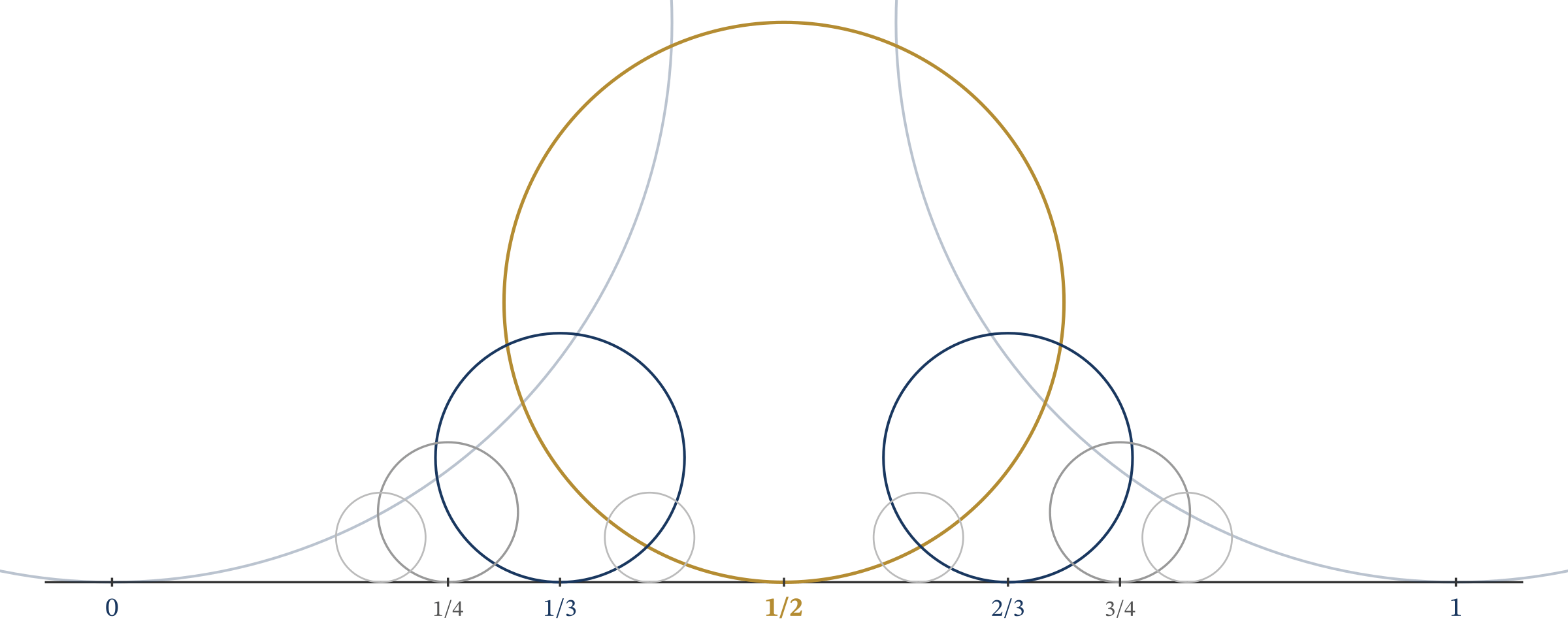
Definition. For a fraction $ p/q $ in lowest terms (with $ q > 0 $), the Ford circle $ C(p,q) $ is the circle with center $ (p/q,\, 1/(2q^2)) $ and radius $ 1/(2q^2) $. It is tangent to the $ x $-axis at the point $ (p/q, 0) $.

[Image: Ford circles for small-denominator fractions, showing tangent circles corresponding to Farey neighbors]

Theorem. Two Ford circles $ C(a,b) $ and $ C(c,d) $ are tangent to each other if and only if $ |ad – bc| = 1 $, i.e., $ a/b $ and $ c/d $ are Farey neighbors.

This beautiful geometric picture connects to continued fractions because consecutive convergents $ p_{n-1}/q_{n-1} $ and $ p_n/q_n $ always satisfy $ |p_n q_{n-1} – p_{n-1} q_n| = 1 $ (the fundamental identity), so their Ford circles are always tangent.

The smaller the denominator of a fraction, the larger its Ford circle. The circle for $ 0/1 $ and $ 1/1 $ have radius $ 1/2 $ and are the largest. The circle for $ 1/2 $ has radius $ 1/8 $ and is tangent to both. As you zoom in, the pattern reveals an intricate fractal-like arrangement that encodes the entire structure of rational approximation.

Farey Sequences

Definition. The Farey sequence $ F_n $ of order $ n $ is the ascending sequence of all fractions $ a/b $ with $ 0 \leq a/b \leq 1 $, $ \gcd(a,b) = 1 $, and $ 0 < b \leq n $.

Example. The first few Farey sequences:

$$ \begin{aligned} F_1 &= \left\{\frac{0}{1}, \frac{1}{1}\right\}\\[4pt] F_2 &= \left\{\frac{0}{1}, \frac{1}{2}, \frac{1}{1}\right\}\\[4pt] F_3 &= \left\{\frac{0}{1}, \frac{1}{3}, \frac{1}{2}, \frac{2}{3}, \frac{1}{1}\right\}\\[4pt] F_4 &= \left\{\frac{0}{1}, \frac{1}{4}, \frac{1}{3}, \frac{1}{2}, \frac{2}{3}, \frac{3}{4}, \frac{1}{1}\right\}\\[4pt] F_5 &= \left\{\frac{0}{1}, \frac{1}{5}, \frac{1}{4}, \frac{1}{3}, \frac{2}{5}, \frac{1}{2}, \frac{3}{5}, \frac{2}{3}, \frac{3}{4}, \frac{4}{5}, \frac{1}{1}\right\} \end{aligned} $$

Theorem (Farey Neighbor Property). If $ a/b $ and $ c/d $ are consecutive fractions in $ F_n $, then $ |bc – ad| = 1 $. Moreover, the next fraction inserted between them is their mediant $ (a+c)/(b+d) $.

This connects directly to Ford circles: consecutive Farey fractions correspond to tangent Ford circles.

The Stern-Brocot Tree

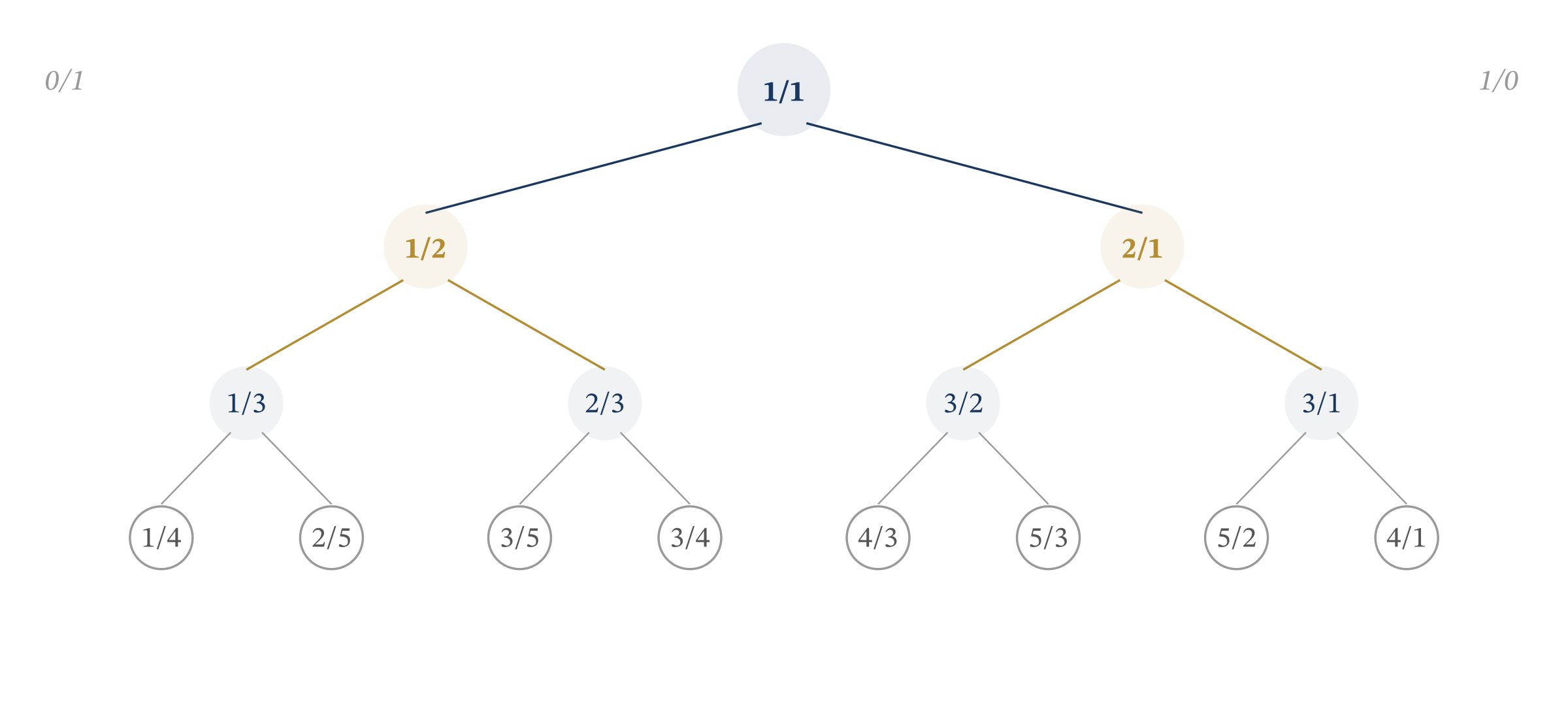
The Stern-Brocot tree is a binary tree that contains every positive rational number exactly once, in lowest terms, organized by the mediant operation.

Definition (Mediant). The mediant of two fractions $ a/b $ and $ c/d $ (with $ b, d > 0 $) is

$$ \frac{a+c}{b+d}. $$

Starting from the “endpoints” $ 0/1 $ and $ 1/0 $ (the latter being a formal symbol for $ \infty $), the tree is built recursively: the root is the mediant $ 1/1 $, and at each node $ p/q $, the left child is the mediant of $ p/q $ with its left ancestor, and the right child is the mediant with its right ancestor.

[Image: The first four levels of the Stern-Brocot tree, showing every positive rational appearing exactly once]

Connection to Continued Fractions

The path from the root to a rational $ p/q $ in the Stern-Brocot tree encodes its continued fraction. If we record “L” for each left turn and “R” for each right turn, and group consecutive identical turns, the group sizes give the partial quotients.

Example. The fraction $ 7/5 $ has CF $ [1; 2, 2] $. In the Stern-Brocot tree, the path is $ R, L, L, R, R $, grouping as $ R^1 L^2 R^2 $, and the exponents $ 1, 2, 2 $ are the partial quotients.

The Gauss-Kuzmin Distribution

A remarkable connection between continued fractions and ergodic theory was initiated by Gauss. The Gauss map $ T: (0,1] \to (0,1] $ defined by $ T(x) = \{1/x\} $ (fractional part of $ 1/x $) is precisely the CF algorithm iterated.

Theorem (Gauss, 1800; Kuzmin, 1928). The Gauss map preserves the probability measure

$$ d\mu = \frac{1}{\ln 2} \cdot \frac{dx}{1+x}. $$

Consequently, for “almost all” real numbers, the partial quotient $ a_n = k $ occurs with asymptotic frequency

$$ \Pr[a_n = k] = \log_2\!\left(1 + \frac{1}{k(k+2)}\right) = \log_2\frac{(k+1)^2}{k(k+2)}. $$

The most common partial quotient is 1, occurring about 41.5% of the time. Then $ a_n = 2 $ occurs about 16.9%, $ a_n = 3 $ about 9.3%, and so on.

Khinchin’s Constant and Levy’s Constant

Theorem (Levy, 1935; Khinchin, 1935). For almost all real numbers $ \alpha = [a_0; a_1, a_2, \ldots] $:

(i) The geometric mean of the partial quotients converges:

$$ \lim_{n \to \infty} (a_1 a_2 \cdots a_n)^{1/n} = K_0 \approx 2.6854520\ldots $$

This is Khinchin’s constant.

(ii) The denominators of convergents grow at a definite rate:

$$ \lim_{n \to \infty} q_n^{1/n} = e^{\pi^2/(12 \ln 2)} \approx 3.2758229\ldots $$

This is Levy’s constant.

Tip: It is unknown whether specific constants like $ \pi $, $ e $, or $ \sqrt{2} $ satisfy Khinchin’s theorem. For $ \sqrt{2} = [1; \overline{2}] $, the geometric mean of partial quotients is just 2, not $ K_0 $. The theorem applies to “generic” numbers, not specific ones.

Open Problems

Despite centuries of study, many natural questions about continued fractions remain open:

Normality of $ \pi $: Are the partial quotients of $ \pi $ distributed according to the Gauss-Kuzmin law?
Bounded partial quotients of algebraic numbers: Is it true that every algebraic irrational of degree $ \geq 3 $ has unbounded partial quotients? This is widely believed but unproven. We do not even know whether the partial quotients of $ \sqrt[3]{2} = [1; 3, 1, 5, 1, 1, 4, 1, 1, 8, \ldots] $ are unbounded.
The Zaremba conjecture: There exists an absolute constant $ A $ such that for every positive integer $ q $, there is a fraction $ p/q $ (in lowest terms) whose partial quotients are all at most $ A $. Bourgain and Kontorovich (2014) proved this for a density-one set of integers $ q $.
Statistics of Pell solutions: How are the period lengths of $ \sqrt{D} $ distributed as $ D $ varies? They seem to grow roughly as $ \sqrt{D} $, but a precise theorem is lacking.

Exercises

Compute the first 8 convergents of $ e = [2; 1, 2, 1, 1, 4, 1, 1, 6, \ldots] $ and verify that convergents just before the large partial quotients give especially good approximations.
Draw (or describe) the Ford circles for the fractions $ 0/1 $, $ 1/1 $, $ 1/2 $, $ 1/3 $, $ 2/3 $. Verify that tangent circles correspond to pairs with $ |ad – bc| = 1 $.
Write out the Farey sequence $ F_6 $ and verify the neighbor property for three consecutive pairs.
Starting from the root $ 1/1 $ of the Stern-Brocot tree, trace the path to $ 5/3 $. Read off the sequence of L’s and R’s, group them, and verify you get the CF $ [1; 1, 2] $.
Using the Gauss-Kuzmin distribution, compute $ \Pr[a_n = 1] + \Pr[a_n = 2] + \Pr[a_n = 3] $. What fraction of partial quotients (for a “typical” number) are at most 3?
Verify Ramanujan’s identity $ R(e^{-2\pi}) = \sqrt{(5 + \sqrt{5})/2} – (1+\sqrt{5})/2 $ numerically by computing the left-hand side to several decimal places.
Use Lambert’s CF for $ \tan x $ with $ x = 1 $ to compute several convergents and compare with $ \tan 1 \approx 1.5574 $.