Geometry and the Chakravala Method - Bhaskaracharya's Lilavati Course

The Lilavati contains a substantial treatment of geometry covering triangles, quadrilaterals, circles, and solid figures. But Bhaskara’s mathematical legacy extends well beyond the Lilavati itself: his algebraic work in the Bijaganita includes the Chakravala method for solving Pell’s equation, and the astronomical sections of the Siddhanta Shiromani contain ideas that anticipate differential calculus by 500 years. This lesson explores Bhaskara’s geometry, his extraordinary Chakravala algorithm, and the concepts that place him among the greatest mathematicians of any era.

The Chakravala method

The broken bamboo problem

Plane Geometry in the Lilavati

Triangles and Heron’s Formula

Bhaskara presents the formula for the area of a triangle with sides $ a $, $ b $, and $ c $:

$$ A = \sqrt{s(s-a)(s-b)(s-c)} $$

where $ s = \frac{a+b+c}{2} $ is the semi-perimeter.

Tip: This formula was known in India before Heron of Alexandria (c. 10-70 CE). Indian mathematicians attribute it to earlier traditions. Bhaskara’s contribution was a particularly elegant proof and systematic presentation.

[Image: Geometric constructions central to the Lilavati, including right triangles, cyclic quadrilaterals, circles, and trapezoids]

The Shadow of the Gnomon

Chapter 9 of the Lilavati applies geometry to astronomical measurements using shadow calculations. A gnomon is a vertical stick whose shadow length changes with the sun’s position.

If a gnomon of height $ h $ casts a shadow of length $ s $, then the altitude angle $ \alpha $ of the sun satisfies:

$$ \tan \alpha = \frac{h}{s} $$

Bhaskara shows how to calculate solar angles, time, and geographical latitude from shadow measurements. This practical application connected pure geometry to everyday life and astronomical observation.

Areas and Volumes

Bhaskara covers volumes and surface areas of three-dimensional shapes including spheres, cones, and pyramids. He uses two approximations for $ \pi $:

$ \pi \approx \frac{22}{7} $ for rough calculations
$ \pi \approx \frac{355}{113} $ for precise work

The area of a circle of radius $ r $:

$$ A = \pi r^2 $$

The volume of a sphere of radius $ r $:

$$ V = \frac{4}{3}\pi r^3 $$

These formulas, stated with the understanding that $ \pi $ is irrational (Bhaskara knew this), demonstrate the practical computational approach of Indian mathematics.

Bhaskara’s Sine Approximation

In the astronomical part of the Siddhanta Shiromani, Bhaskara provides a remarkably accurate rational approximation for the sine function:

Important: Bhaskara I’s Sine Approximation (later refined by Bhaskara II):
$ \sin\theta \approx \frac{16\theta(\pi – \theta)}{5\pi^2 – 4\theta(\pi – \theta)} $, for $ 0 \leq \theta \leq \pi $
This formula achieves a maximum error of less than 1.9% over the entire range.

At the key values:

For $ \theta = \frac{\pi}{6} $: the formula gives exactly $ \frac{1}{2} $. Correct.

For $ \theta = \frac{\pi}{2} $: the formula gives

$$ \frac{16 \cdot \frac{\pi}{2} \cdot \frac{\pi}{2}}{5\pi^2 – 4 \cdot \frac{\pi}{2} \cdot \frac{\pi}{2}} = \frac{4\pi^2}{5\pi^2 – \pi^2} = \frac{4\pi^2}{4\pi^2} = 1 $$

Also exact. The formula is a rational function that closely approximates the transcendental sine function, a remarkable achievement for the 12th century.

The Chakravala Method

Though appearing more fully in Bhaskara’s algebraic work (Bijaganita), the Chakravala method represents one of the greatest algorithmic achievements of Indian mathematics.

Pell’s Equation

Pell’s equation is the Diophantine equation:

$$ x^2 – Dy^2 = 1 $$

where $ D $ is a given positive non-square integer, and integer solutions $ (x, y) $ are sought.

Tip: Despite the name, Pell’s equation was not studied by John Pell. The misnomer was introduced by Euler, who attributed it to Pell. Indian mathematicians, particularly Brahmagupta (628 CE) and Bhaskara II, developed the theory centuries before any European work on the problem.

The Algorithm

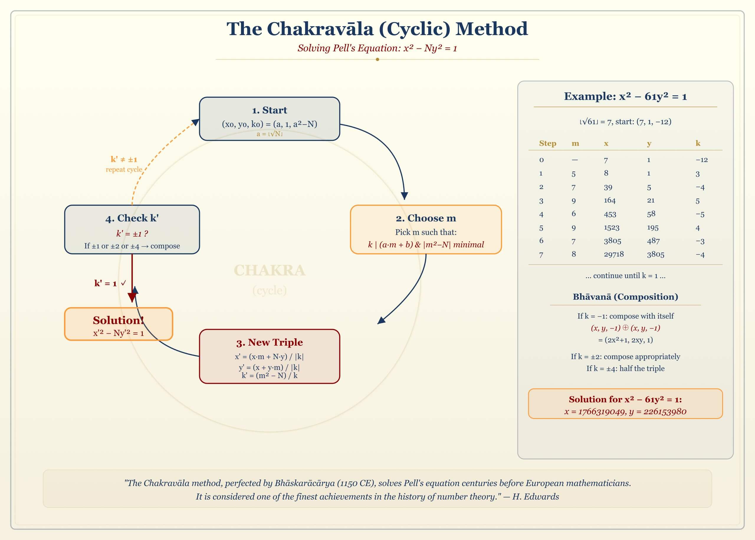
The Chakravala (“cyclic method”) solves $ x^2 – Dy^2 = 1 $ through the following iterative process:

[Image: The Chakravala cyclic method, showing an iterative algorithm for solving Pell’s equation]

Start with an initial triple $ (x_0, y_0, k_0) $ where $ x_0^2 – Dy_0^2 = k_0 $ and $ |k_0| $ is small.
At each step, find $ m $ such that:
- $ k_i \mid (x_i + m y_i) $
- $ |m^2 – D| $ is minimized
Compute the next triple:

$$ x_{i+1} = \frac{x_i m + D y_i}{|k_i|}, \quad y_{i+1} = \frac{x_i + m y_i}{|k_i|}, \quad k_{i+1} = \frac{m^2 – D}{k_i} $$

Repeat until $ k_i = 1 $.

The key insight is the composition identity (known to Brahmagupta):

If $ x_1^2 – Dy_1^2 = k_1 $ and $ x_2^2 – Dy_2^2 = k_2 $, then

$$ (x_1 x_2 + D y_1 y_2)^2 – D(x_1 y_2 + x_2 y_1)^2 = k_1 k_2 $$

This identity, called the Brahmagupta-Bhaskara identity or the samasa (composition), is the engine that powers the Chakravala method. It allows one to combine two “near-solutions” to produce a better one.

Worked Example: Solving $ x^2 – 61y^2 = 1 $

This is one of Bhaskara’s own examples in the Bijaganita. We trace the Chakravala algorithm.

Step 0: Start with $ (x_0, y_0, k_0) = (8, 1, 3) $ since $ 8^2 – 61 \cdot 1^2 = 64 – 61 = 3 $.

Step 1: Find $ m $ such that $ 3 \mid (8 + m) $ and $ |m^2 – 61| $ is minimized. The candidates satisfying $ 8 + m \equiv 0 \pmod{3} $ are $ m = 1, 4, 7, 10, \ldots $ We check: $ |1 – 61| = 60 $, $ |16 – 61| = 45 $, $ |49 – 61| = 12 $, $ |100 – 61| = 39 $. Minimum at $ m = 7 $.

New triple:

$$ x_1 = \frac{8 \cdot 7 + 61 \cdot 1}{3} = \frac{117}{3} = 39, \quad y_1 = \frac{8 + 7}{3} = 5, \quad k_1 = \frac{49 – 61}{3} = -4 $$

Check: $ 39^2 – 61 \cdot 25 = 1521 – 1525 = -4 $. Correct.

The algorithm continues through several more steps, eventually reaching $ k = 1 $. The final solution is:

$$ x = 1766319049, \quad y = 226153980 $$

Verification: $ 1766319049^2 – 61 \times 226153980^2 = 1 $.

The fact that Bhaskara could find this enormous solution demonstrates the power of the Chakravala algorithm. The method was not rediscovered in Europe until Lagrange’s work in 1768, over 600 years later.

Why the Chakravala Works

The Chakravala method can be understood in modern terms through the theory of continued fractions. The solutions to Pell’s equation are given by the convergents of the continued fraction expansion of $ \sqrt{D} $. The Chakravala algorithm essentially computes these convergents, but through a different route: instead of computing the continued fraction directly, it uses Brahmagupta’s composition identity to combine approximate solutions.

The choice of $ m $ that minimizes $ |m^2 – D| $ at each step corresponds to choosing the best rational approximation to $ \sqrt{D} $, which is exactly what continued fractions do. The condition $ k_i \mid (x_i + my_i) $ ensures that the new triple has integer entries.

Early Differential Calculus

In the astronomical sections of the Siddhanta Shiromani, Bhaskara computes what we would now call the derivative of $ \sin\theta $.

Important: Bhaskara’s Proto-Derivative: Bhaskara observed that the “instantaneous velocity” of a sine function is proportional to the cosine:
$ \frac{\delta(\sin\theta)}{\delta\theta} \approx \cos\theta $
This result, expressed in the context of planetary motion, predates Newton and Leibniz by over 500 years.

Bhaskara’s reasoning was as follows: if a planet’s angular position follows a sinusoidal pattern (as it does in the Indian epicyclic model), then the rate of change of its position at any instant is given by the cosine of the angle. He expressed this as: “the difference of the sines is the product of the difference of the arcs and the cosine, divided by the radius.”

In modern notation, this is:

$$ \sin(\theta + \delta) – \sin\theta \approx \delta \cdot \cos\theta $$

for small $ \delta $, which is precisely the statement that $ \frac{d}{d\theta}\sin\theta = \cos\theta $.

Bhaskara also understood the concept that at a maximum (or minimum) of a function, the instantaneous rate of change is zero. He noted that the sine function has zero rate of change at $ \theta = \frac{\pi}{2} $, where indeed $ \cos\frac{\pi}{2} = 0 $.

Iterative Algorithms

Bhaskara’s methods for calculating square roots and solving equations use iterative refinement, anticipating numerical methods used in modern computer algorithms.

Iterative Square Root. Starting with approximation $ a_0 $, the iteration:

$$ a_{n+1} = \frac{1}{2}\left(a_n + \frac{N}{a_n}\right) $$

converges to $ \sqrt{N} $. This is the Babylonian method, known in India from ancient times and presented by Bhaskara with improved convergence analysis.

The convergence is quadratic: the number of correct digits roughly doubles at each step. Starting from $ a_0 = 8 $ to compute $ \sqrt{61} $:

$$ \begin{aligned} a_0 &= 8 \\ a_1 &= \frac{1}{2}\left(8 + \frac{61}{8}\right) = \frac{1}{2} \cdot \frac{125}{8} = 7.8125 \\ a_2 &= \frac{1}{2}\left(7.8125 + \frac{61}{7.8125}\right) \approx 7.81025 \\ \end{aligned} $$

The true value is $ \sqrt{61} \approx 7.81025 $, so after just two iterations we have 5-digit accuracy.

Lilavati’s Influence on World Mathematics

Transmission to the Islamic World

Persian translations of the Lilavati appeared in the 13th century. The translator Abu’l Faiz Faizi produced a notable Persian version in 1587 at the court of the Mughal Emperor Akbar.

Influence on European Mathematics

From the Islamic world, Indian mathematical concepts filtered into European mathematics. Fibonacci, whose work popularized Hindu-Arabic numerals in Europe, likely encountered Indian mathematical ideas through Arabic intermediaries.

The decimal place-value system, the concept of zero, and algorithms for arithmetic operations, all developed in India and transmitted through Arabic scholars, form the foundation of modern computation.

Educational Legacy

The pedagogical approach in the Lilavati influenced how mathematics was taught:

The use of engaging word problems to motivate abstract concepts
Progression from simple to complex topics
Integration of practical applications with theoretical foundations
The practice of providing worked examples before exercises

These are now considered educational best practices, and Bhaskara was using them in the 12th century. In India, the Lilavati remained in classroom use well into the 19th century.

The Lilavati in Modern Perspective

Many problem types from the Lilavati appear in modern textbooks and competitions:

Work-rate problems (pipes and cisterns)
Mixture problems
Pursuit problems (the peacock and the snake)
Number puzzles (the maiden’s riddle)
Combinatorial counting

The mathematical structures underlying these problems, including linear equations, quadratic equations, the Pythagorean theorem, and arithmetic and geometric series, form the core of secondary mathematics education worldwide.

Summary of Bhaskara’s Key Contributions

Systematic Arithmetic: Complete treatment of the four operations, fractions, zero, and negative numbers.
Elegant Problem Design: Mathematical problems embedded in memorable stories about bees, peacocks, lotuses, and maidens.
Algorithmic Thinking: The Kuttaka and Chakravala methods represent algorithmic sophistication not matched in Europe for centuries.
Proto-Calculus: Computation of instantaneous rates of change anticipated differential calculus by 500 years.
Educational Innovation: A pedagogical approach that made mathematics accessible, engaging, and memorable.

As we solve the problems of the Lilavati today, we connect with a mathematical tradition that stretches back nearly a millennium, and find that the human desire to understand the world through numbers and patterns is truly timeless.

Exercises

A triangle has sides 13, 14, and 15. Use Heron’s formula to find its area.
A gnomon of height 12 units casts a shadow of length 5 units. What is the altitude angle of the sun? Express your answer in degrees.
Use the Chakravala method to solve $ x^2 – 7y^2 = 1 $. Start with the initial triple $ (3, 1, 2) $ since $ 9 – 7 = 2 $. (The smallest solution is $ x = 8, y = 3 $.)
Verify Brahmagupta’s composition identity: if $ 8^2 – 61 \cdot 1^2 = 3 $ and $ 39^2 – 61 \cdot 5^2 = -4 $, compose them to obtain a new solution to $ x^2 – 61y^2 = k $ for some $ k $. (Use the formula $ (x_1 x_2 + Dy_1 y_2, x_1 y_2 + x_2 y_1) $.)
Using Bhaskara’s sine approximation formula, compute $ \sin(\pi/4) $ and compare with the exact value $ \frac{\sqrt{2}}{2} \approx 0.7071 $.
Apply the iterative square root method to compute $ \sqrt{10} $, starting from $ a_0 = 3 $. Perform 3 iterations and compare with the true value $ \sqrt{10} \approx 3.16228 $.
The Pell equation $ x^2 – 2y^2 = 1 $ has solutions $ (3, 2) $, $ (17, 12) $, $ (99, 70) $, etc. Verify that each can be obtained from the previous by Brahmagupta’s composition identity.
A sphere has surface area $ 616 $ square units. Using $ \pi = \frac{22}{7} $, find the radius and volume in the style of Bhaskara.
Bhaskara says the derivative of $ \sin\theta $ is $ \cos\theta $. Using the limit definition, verify that $ \lim_{\delta \to 0} \frac{\sin(\theta + \delta) – \sin\theta}{\delta} = \cos\theta $. (Hint: use the angle addition formula and the limits $ \lim_{x \to 0} \frac{\sin x}{x} = 1 $ and $ \lim_{x \to 0} \frac{\cos x – 1}{x} = 0 $.)
Research problem: The Kerala school (Madhava, c. 1400 CE) later developed infinite series for $ \pi $ and trigonometric functions, building on the Indian mathematical tradition that includes Bhaskara. The Madhava-Leibniz series is $ \frac{\pi}{4} = 1 – \frac{1}{3} + \frac{1}{5} – \frac{1}{7} + \cdots $. Compute the first 10 partial sums and observe the convergence rate.