Analysis of Meteorological Data of Pantnagar Weather Station

This paper presents a statistical analysis of 20 years of meteorological data (1989-2008) from the Pantnagar weather station in Uttarakhand, India. The research was conducted under the INSPIRE-SHE Scholarship Program, Department of Science and Technology, Government of India. The goal: extract meaningful patterns from atmospheric data using regression analysis, correlation studies, and time-series methods.

Abstract

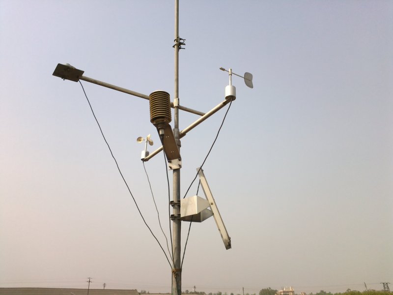
Twenty years of weekly meteorological observations from the IMD-approved weather station at Govind Ballabh Pant University of Agriculture and Technology, Pantnagar, were analyzed to characterize the regional climate and assess parameter variability. The observatory is located at 29°N latitude, 79.3°E longitude, and 243.84 m altitude in the Tarai belt of Uttarakhand.

Key findings: Annual rainfall averages 1610.8 mm with extreme variability (σ = 2768.4 mm). Mean annual maximum temperature is 29.6°C (σ = 0.575°C), while mean annual minimum is 16.9°C (σ = 0.344°C). The region experiences dramatic diurnal humidity swings, from 84.7% (morning) to 50.8% (afternoon). Regression and correlation analyses reveal weak coupling between rainfall magnitude and rainy-day count, confirming the stochastic nature of precipitation in this region.

Keywords: meteorology, Pantnagar, regression analysis, rainfall variability, Tarai climate, time-series analysis

1. Introduction

Meteorology, from the Greek “meteoros” (atmospheric) and “logos” (science), is the study of atmospheric processes through applied physics. The science encompasses both static and dynamic components of the atmosphere, collectively termed weather.

Understanding regional climate patterns requires long-term observational data. Short-term records capture noise. Twenty years of data, like the dataset analyzed here, can reveal underlying trends while accounting for natural variability.

The Pantnagar region presents a unique study area. Located in the Tarai belt at the base of the Himalayan foothills, it experiences extreme seasonal variation: summer temperatures exceeding 42°C and winter lows near 2°C. Annual rainfall averages 145 cm, concentrated in a four-month monsoon season (June-September). The alluvial soil, with pH 7.2-7.4, supports intensive agriculture, making meteorological prediction economically critical for the region.

1.1 Study Objectives

This research aimed to:

1. Characterize the statistical distribution of key meteorological parameters
2. Quantify inter-annual variability in temperature, rainfall, and humidity
3. Identify correlations between meteorological variables
4. Develop regression models for parameter estimation
5. Apply moving-average techniques to identify long-term trends

2. Theoretical Background

2.1 Atmospheric Structure

Earth’s atmosphere is a thin gaseous envelope bound by gravity. Its composition: nitrogen (78%), oxygen (21%), and trace gases including argon and carbon dioxide (~1%). Variable constituents, water vapor, ozone, and particulate matter, vary by location and time, driving weather phenomena.

The atmosphere stratifies into distinct layers:

Troposphere (0-8/16 km): Contains three-fourths of atmospheric mass and nearly all moisture and dust. All weather phenomena occur here. Temperature decreases with altitude at the lapse rate of approximately 6.5°C/km. The tropopause height varies from 8 km at poles to 16 km at the equator.

Stratosphere (tropopause to 50 km): Stable, moisture-free layer containing the ozone shield. Temperature increases with altitude due to UV absorption by ozone.

Mesosphere (50-80 km): Temperature decreases with altitude. The mesopause marks the coldest point in the atmosphere.

Ionosphere/Thermosphere (80-600 km): Extremely low pressure (~0.01 mbar at 90 km). Contains ionized particles that reflect radio waves.

Exosphere (>600 km): The atmosphere gradually merges into interplanetary space. Mean free path becomes very large.

Note: Meteorological studies focus primarily on the troposphere, with extension into the stratosphere for ozone-related research.

2.2 Meteorological Parameters

Weather stations record multiple parameters at standardized times (07:12 and 14:12 hours IST for Indian stations). The parameters relevant to this study:

Atmospheric Pressure

Atmospheric pressure is the force exerted per unit area by the column of air above a location. Measured using Fortin’s barometer (mercury column) or aneroid barometer. Continuous recording uses a barograph.

Standard atmospheric pressure: \( 1.013 \times 10^5 \) N/m² (1 atm = 1013.25 hPa)

Wind Direction and Velocity

Wind refers to horizontal air movement parallel to Earth’s surface. Vertical components are termed air currents. Direction is measured by wind vane; velocity by cup anemometer.

Temperature

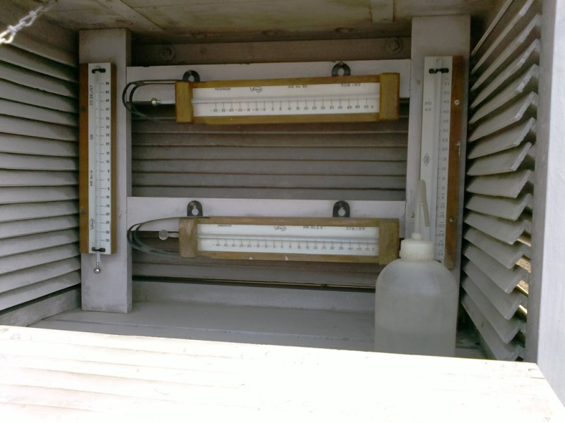
The most fundamental meteorological parameter. Measured using mercury thermometers; continuous recording via thermograph (bimetallic strip principle). Key derived quantities:

• Mean daily temperature: Arithmetic average of daily maximum and minimum
• Daily range: Difference between maximum and minimum temperatures
• Mean monthly temperature: Average of all daily means in a month
• Normal temperature: 30-year average (climatological standard)

Humidity

Relative humidity measures the ratio of actual vapor pressure to saturation vapor pressure at a given temperature, expressed as a percentage. Measured using psychrometer (wet-bulb/dry-bulb thermometer pair). Continuous recording via hygrograph.

Radiation

Solar radiation drives atmospheric dynamics. Thermal radiation affects surface temperature. Both influence evaporation rates and cloud formation.

Sunshine Duration

Hours of bright sunshine per day, measured by Campbell-Stokes sunshine recorder (glass sphere focusing sunlight to burn a trace on calibrated card).

Precipitation

All forms of atmospheric water deposition: rainfall, snowfall, hail, fog. Rainfall measured using rain gauges. Three methods for computing areal averages:

1. Arithmetic Mean Method (used in this study):

$$\bar{P} = \frac{1}{n} \sum_{k=1}^{n} P_k$$

where \( P_k \) represents rainfall at station \( k \) and \( n \) is the number of stations.

2. Thiessen Polygon Method:

$$\bar{P} = \frac{\sum_{k=1}^{n} A_k P_k}{\sum_{k=1}^{n} A_k}$$

where \( A_k \) is the polygonal area around station \( k \). Accounts for irregular station spacing.

3. Isohyetal Method: Contour mapping of equal rainfall lines. Most accurate but requires analyst skill.

Evaporation

Water loss from surfaces due to vaporization. Measured using pan evaporimeters (standard water tank with depth gauge). Critical for water resource management and agricultural planning.

3. Methodology

3.1 Data Source and Period

Weekly meteorological data spanning 1989-2008 (20 years) were obtained from the Agro-Meteorological Observatory at G.B. Pant University of Agriculture and Technology, Pantnagar. The observatory operates under the N.E.B. Crop Research Center and is IMD-approved.

Observations recorded twice daily (07:12 and 14:12 hours), yielding 14 observations per week. Analysis was performed on weekly aggregated data.

3.2 Statistical Framework

Meteorological phenomena are predominantly stochastic. Unlike deterministic processes (sunrise, sunset), most weather parameters exhibit inherent unpredictability. This requires probabilistic treatment.

Key definitions:

Probability: If an experiment is conducted \( N \) times and outcome \( A \) occurs \( n \) times:

$$P(A) = \lim_{N \to \infty} \frac{n}{N}$$

Probability ranges from 0 (impossible) to 1 (certain).

Random Variable: A variable associated with a stochastic process whose value cannot be predicted deterministically. Denoted by uppercase letters (X); specific values by lowercase (x).

• Discrete random variable: Takes countable values (e.g., number of rainy days)
• Continuous random variable: Takes values on a continuum (e.g., rainfall amount)

3.3 Regression Analysis

Regression analysis has been fundamental to Indian monsoon prediction since Blanford (1884), refined by Sir Gilbert Walker (1921-1927). Three regression types were considered:

Simple Linear Regression:

$$y = a + bx$$

where \( x \) is the independent variable, \( y \) is the dependent variable, and \( a \), \( b \) are regression constants.

Multiple Linear Regression:

$$y = a_0 + a_1 x_1 + a_2 x_2 + \cdots + a_n x_n$$

for \( n \) independent variables.

Curvilinear Regression:

$$y = ax^b$$

Linearized via logarithmic transformation: \( \log y = \log a + b \log x \)

Least Squares Estimation

For observations \( (x_1, y_1), (x_2, y_2), \ldots, (x_n, y_n) \), optimal regression coefficients minimize the sum of squared residuals:

$$S = \sum_{k=1}^{n} (y_k – a – bx_k)^2$$

Setting partial derivatives to zero yields the normal equations:

$$\frac{\partial S}{\partial a} = 0 \quad \text{and} \quad \frac{\partial S}{\partial b} = 0$$

For multiple regression with \( n \) predictors:

$$S = \sum_{k=1}^{N} \left( y_k – a_0 – \sum_{j=1}^{n} a_j x_{jk} \right)^2$$

This generates \( n+1 \) normal equations.

3.4 Correlation Analysis

The Pearson correlation coefficient quantifies linear association between variables:

$$r = \frac{\frac{1}{n} \sum_{k=1}^{n} (x_k – \bar{x})(y_k – \bar{y})}{s_x \cdot s_y}$$

where \( \bar{x} \), \( s_x \) and \( \bar{y} \), \( s_y \) are means and standard deviations of variables \( X \) and \( Y \) respectively.

Interpretation:

• \( r = +1 \): Perfect positive correlation
• \( r = -1 \): Perfect negative correlation
• \( r = 0 \): No linear correlation

3.5 Software Tools

Analysis was performed using SPSS (statistical analysis and graphing), Mathematica (complex calculations), Microsoft Excel (data manipulation and moving averages), and LaTeX (document preparation).

4. Results

4.1 Temperature Analysis

Temperature exhibited the lowest inter-annual variability among all parameters studied.

Annual Maximum Temperature:

• Mean: \( \bar{T}_{max} = 29.6 \)°C
• Standard deviation: \( s_{T_{max}} = 0.575 \)°C
• Range: 28.3°C to 30.4°C

Annual Minimum Temperature:

• Mean: \( \bar{T}_{min} = 16.9 \)°C
• Standard deviation: \( s_{T_{min}} = 0.344 \)°C
• Range: 16.3°C to 17.5°C

Weekly Extremes:

• Maximum recorded: 42°C (summer)
• Minimum recorded: 2.4°C (winter)

The contrast between low inter-annual variability (σ < 0.6°C) and high intra-annual range (~40°C) is characteristic of continental Tarai climate.

4.2 Rainfall Analysis

Rainfall exhibited extreme variability, confirming its stochastic nature.

Annual Rainfall:

• Mean: \( \bar{P} = 1610.8 \) mm/year
• Standard deviation: \( s_P = 2768.4 \) mm/year
• Minimum year: 831.2 mm (1992)
• Maximum year: 3218.6 mm (2000)

The coefficient of variation (CV = σ/μ = 1.72) indicates extreme inter-annual variability.

Rainy Days:

• Mean: 78 days/year
• Standard deviation: 11.8 days/year
• Range: 63 to 100 days

Critical finding: Weak correlation between total rainfall and number of rainy days. This implies high uncertainty in daily precipitation intensity, even when rainy-day count is known.

4.3 Humidity Analysis

Dramatic diurnal variation, characteristic of the Tarai belt:

Morning (07:12 hrs):

• Mean: 84.7%
• Range: 81.7% to 86.9%

Afternoon (14:12 hrs):

• Mean: 50.8%
• Range: 44.5% to 56.0%

The 34 percentage-point average diurnal swing reflects rapid morning evaporation in the subtropical climate.

4.4 Additional Parameters

Sunshine Duration:

• Mean: 7.37 hours/day
• Range: 6.40 hrs (2008) to 7.97 hrs (1989)

Wind Velocity:

• Annual mean: 4.75 km/h
• Annual range: 2.94 to 7.03 km/h
• Daily range: 0.8 to 30 km/h

Evaporation:

• Mean: 4.85 mm/day
• Range: 3.92 to 5.41 mm/day

5. Discussion

5.1 Climate Characterization

The Pantnagar climate exhibits three defining characteristics:

1. Temperature Stability with Extreme Seasonality: Year-to-year mean temperatures vary by less than 1°C, yet seasonal range exceeds 40°C. This allows reliable agricultural planning while demanding crop varieties tolerant of both heat and cold stress.

2. Rainfall Unpredictability: The coefficient of variation of 1.72 for annual rainfall indicates that rainfall in any given year may deviate from the mean by more than 170%. This extreme variability poses significant challenges for water resource management and rain-fed agriculture.

3. Humidity Dynamics: The 34-point diurnal humidity swing affects evapotranspiration rates, irrigation scheduling, and pest/disease prevalence. Morning conditions favor fungal growth; afternoon conditions promote rapid drying.

5.2 Methodological Considerations

The arithmetic mean method for rainfall averaging, while simplest, assumes uniform station weighting. For a single-station dataset like this, the limitation is moot. For regional studies, Thiessen polygon or isohyetal methods would provide superior accuracy.

Moving average analysis (3-year and 5-year windows) revealed no statistically significant long-term trends in temperature or rainfall over the 20-year period. This suggests climate stationarity during 1989-2008, though longer records would be needed to assess climate change impacts.

6. Conclusions

Analysis of 20 years of meteorological data from Pantnagar reveals:

1. Temperature: Highly predictable on annual basis (σ < 0.6°C) despite extreme seasonal variation (range ~40°C).
2. Rainfall: Highly unpredictable (CV = 1.72). Weak correlation with rainy-day count indicates intensity uncertainty even when occurrence is known.
3. Humidity: Consistent diurnal pattern with ~34% swing from morning to afternoon.
4. Sunshine and Evaporation: Relatively stable parameters with low inter-annual variability.
5. Wind: Low mean velocity (4.75 km/h) with high daily variability.

These findings support the classification of Pantnagar as a humid subtropical climate with monsoon characteristics and extreme rainfall variability typical of the Indo-Gangetic Tarai belt.

Data Availability

The following datasets are available for download:

• Complete 20-year weekly meteorological data (1989-2008)
• Yearly data with analytical graphs and moving averages
• Rainfall moving average calculations
• Temperature moving average calculations

Acknowledgments

This research was conducted under the INSPIRE-SHE Scholarship Program, Department of Science and Technology, Government of India. The author thanks the Agro-Meteorological Observatory at G.B. Pant University of Agriculture and Technology, Pantnagar, for providing access to meteorological records.

References

1. Weisner, C.J. (1983). Hydrometeorology. Chapman & Hall Ltd., London.
2. Reddy, P.J. (2006). A Textbook of Hydrology. Laxmi Publications, India.
3. Sharma, M.A. & Singh, J.B. “Use of Probability Distribution in Rainfall Analysis.”
4. Walker, G.T. (1921-1927). Correlation in seasonal variations of weather. Memoirs of the India Meteorological Department.
5. Blanford, H.F. (1884). On the connection of the Himalayan snowfall with dry winds and seasons of drought in India. Proceedings of the Royal Society of London, 37, 3-22.

Frequently Asked Questions