Hopalong Orbits Visualizer: The Math Behind the Most Beautiful WebGL Experiment
Three lines of algebra. That’s all it takes to generate structures that look like they belong in the Hubble Deep Field.
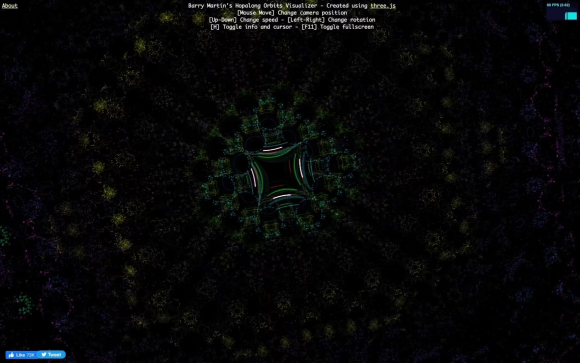
Barry Martin’s Hopalong Orbits Visualizer is a WebGL experiment by Iacopo Sassarini that renders the Hopalong attractor as a 3D point cloud in your browser. Hundreds of thousands of iterated points, colored by position and depth, rotating in real-time on your GPU. The result looks like a luminous nebula. But underneath, it’s just a simple iterative map doing arithmetic over and over.
I’ve been fascinated by this experiment since I first found it years ago. It sits at the intersection of pure mathematics, chaos theory, and generative art. And the math is accessible enough that anyone with high school algebra can understand why it works.
What is the Hopalong attractor?
The Hopalong attractor is a two-dimensional discrete-time dynamical system discovered by Barry Martin at the University of Aston in Birmingham, England. Martin explored these iterative maps in the early 1980s, and they reached a wide audience through A.K. Dewdney’s “Computer Recreations” column in Scientific American in 1986. Dewdney’s column was the successor to Martin Gardner’s legendary “Mathematical Games,” and he presented Martin’s map as proof that extraordinarily complex images could emerge from trivially simple rules.
The map is defined by two equations that update a point \((x, y)\) at each step:
$$ x_{n+1} = y_n – \text{sign}(x_n) \cdot \sqrt{|b \cdot x_n – c|} $$
$$ y_{n+1} = a – x_n $$
Where \(a\), \(b\), and \(c\) are real-valued parameters, and \(\text{sign}(x)\) returns +1 if \(x > 0\), -1 if \(x < 0\), and 0 if \(x = 0\).
That’s it. You pick starting values (usually \(x_0 = 0, y_0 = 0\)), choose three parameters, and iterate. Each step produces a new point. Plot a few hundred thousand of them and you get structures that look like they were designed by an artist, not computed by three lines of arithmetic.
Why the sign function is the key ingredient
Remove the \(\text{sign}(x_n)\) term and the map becomes boring. It’s the sign function that makes the Hopalong attractor hop.
Here’s what it does. The sign function partitions the plane into two half-planes: \(x > 0\) and \(x < 0\). In each half, the map behaves as a different smooth function. When \(x_n\) is positive, the sign term subtracts the square root. When negative, it adds. This forces the orbit to alternate sides, jumping back and forth across the y-axis with each iteration.
That back-and-forth hopping is where the name comes from. And it’s what prevents the orbit from settling into simple periodic behavior. Every time the orbit crosses the y-axis, it gets kicked in a different direction. The result is a trajectory that’s bounded (it never flies off to infinity) but non-periodic (it never exactly repeats). Over thousands of iterations, the orbit densely fills a bounded region of the plane, gradually painting the intricate pattern you see in the visualizer.
This is similar to what happens with other iterative systems in mathematics. The Collatz conjecture, for instance, produces sequences that bounce unpredictably despite following a simple rule. The Hopalong map trades Collatz’s integer arithmetic for real-valued geometry, but the principle is the same: simple rules, complex behavior.
How the parameters shape the pattern
The three parameters \(a\), \(b\), and \(c\) control everything about the visual output. Small changes produce dramatically different patterns.
Parameter \(a\) controls the overall displacement. Since \(y_{n+1} = a – x_n\), the value of \(a\) shifts the center of the pattern vertically. Larger values of \(a\) spread the structure.
Parameter \(b\) scales the x-coordinate inside the square root. It controls the “stretch” of the pattern. When \(b\) is close to 0, the square root term approaches \(\sqrt{|c|}\), becoming nearly constant. The pattern gets more regular and periodic-looking.
Parameter \(c\) acts as an offset inside the square root. When \(c\) is close to 0, the expression simplifies to \(\sqrt{|b \cdot x|}\), and the patterns tend toward more symmetric rosette forms.
One of the most mathematically intriguing properties: certain parameter combinations produce patterns with apparent rotational symmetry (3-fold, 5-fold, 7-fold), even though no rotational symmetry is explicitly encoded in the equations. This emergent symmetry arises from the interaction between the piecewise dynamics and the parameter ratios. Irrational relationships between parameters tend to produce the most complex, space-filling patterns. Rational relationships give more structured, quasi-periodic designs.
Is it actually a “strange attractor”?
Technically, no. And this is worth understanding if you care about the mathematics.
A strange attractor in the strict dynamical systems sense requires dissipation. The system must contract volumes in phase space. The Lorenz attractor (1963) and the Henon map (1976) are dissipative: they have Jacobian determinants with magnitude less than 1, meaning nearby trajectories converge toward the attractor over time.
The Hopalong map is different. It’s area-preserving (conservative). Its Jacobian determinant has magnitude 1. The orbit doesn’t converge toward a fractal set. Instead, it densely fills a bounded region, visiting every part of it given enough iterations. Think of it like a function that’s everywhere continuous but nowhere differentiable: the behavior is well-defined but endlessly intricate at every scale.
| Attractor | Discoverer | Year | Type | Dissipative? |
|---|---|---|---|---|
| Lorenz | Edward Lorenz | 1963 | Continuous (ODE) | Yes |
| Henon | Michel Henon | 1976 | Discrete 2D map | Yes |
| Hopalong/Martin | Barry Martin | ~1982 | Discrete 2D map | No (conservative) |
| Clifford | Clifford Pickover | 1990s | Discrete 2D map | Yes |
| De Jong | Peter de Jong | 1990s | Discrete 2D map | Yes |
In practice, nobody outside a dynamical systems seminar cares about this distinction. The Hopalong map lives in the same aesthetic and mathematical neighborhood as strange attractors, and it’s universally discussed alongside them. The visual output is equally stunning.
How the WebGL visualizer works
Iacopo Sassarini’s visualizer does something clever with the 2D attractor: it maps it into three dimensions.
The process works in four stages:
1. Point generation. The application iterates the Hopalong equations hundreds of thousands of times (typically 100,000 to 1,000,000+ points), starting from \((0, 0)\) with randomized parameters \(a\), \(b\), \(c\). Each iteration produces an \((x, y)\) coordinate pair stored in a buffer.
2. 3D mapping. Here’s the creative leap. Sassarini distributes successive orbit points along a third axis (z), effectively unrolling the flat 2D attractor into a volumetric point cloud. Points land on successive depth planes, so what was a flat pattern gains depth and sculptural form. Multiple orbits with slightly varied parameters are layered together, creating the characteristic galaxy-like appearance.
3. Color mapping. Points are colored based on their position in the iteration sequence and their spatial coordinates. Smooth color gradients sweep across the structure, enhancing depth perception and giving the mathematical object an organic, almost biological quality.
4. GPU rendering. This is where Three.js (created by Ricardo Cabello, aka Mr.doob) comes in. The point cloud is rendered as a WebGL particle system using THREE.Points with a BufferGeometry. Each attractor iterate becomes a vertex. The GPU renders all points in a single draw call with additive blending, so overlapping points create brighter regions. This naturally highlights the denser parts of the orbit, revealing the attractor’s internal structure. A modern GPU handles a million points at 60fps without breaking a sweat.
The camera continuously orbits around the point cloud, providing an ever-changing perspective. You can also interact: zoom, rotate, and explore the structure yourself. The real-time interactivity transforms a static mathematical object into a living, explorable space.

The deeper connection: chaos, beauty, and information
Why do chaotic systems produce beautiful patterns? This isn’t just an aesthetic coincidence. There’s a mathematical reason.
Iterative maps like Martin’s Hopalong are compressed descriptions of visual complexity. A three-line equation generates images that would require millions of explicit drawing instructions. The information content of the image is enormous, but the algorithmic complexity of the generating rule is tiny. This gap between descriptive simplicity and output complexity is what makes these systems both mathematically interesting and visually striking.
The aesthetics arise from the same properties that matter in dynamical systems theory. Self-organization: simple iterative rules spontaneously generate large-scale geometric order (spirals, rosettes, filaments) without any explicit geometric programming. Dense orbits: ergodic-like behavior means the orbit visits every part of the bounded region, gradually painting the pattern with increasing detail. Deterministic chaos: the rules are perfectly deterministic, so the patterns have coherent structure, but the sensitivity to initial conditions means the structure is endlessly intricate.
This is the same principle that makes fractals compelling. The Mandelbrot set emerges from the iteration \(z_{n+1} = z_n^2 + c\). The Poincare conjecture dealt with the topology of spaces that exhibit this kind of structural richness. Martin’s Hopalong shows that you don’t need complex numbers or differential equations to get there. Basic real arithmetic with a sign function is enough.
Try it yourself
The visualizer runs in any modern browser with WebGL support (Chrome, Firefox, Safari, Edge). No plugins, no installation. Just click and watch.
If you want to experiment with the parameters yourself, the map is trivial to implement. Here’s the core loop in pseudocode:
x, y = 0, 0
for i in range(1000000):
    x_new = y - sign(x) * sqrt(abs(b * x - c))
    y_new = a - x
    x, y = x_new, y_new
    plot(x, y)
Try \(a = 1.1\), \(b = 0.5\), \(c = 1.0\) as a starting point. Then nudge the parameters by 0.1 in each direction and watch the pattern transform. You’ll see rosettes, spirals, filaments, and structures that look like they belong on a NASA press release. All from three lines of algebra and a simple iterative process.
That’s the thing about mathematics. The most beautiful results often come from the simplest rules. You don’t need a supercomputer or a PhD. You need a loop, a square root, and the patience to let the pattern reveal itself.
Frequently Asked Questions
What is the Hopalong attractor?
The Hopalong attractor is a two-dimensional iterative map discovered by Barry Martin at the University of Aston, Birmingham. It uses the equations x’ = y − sign(x)·√|bx − c| and y’ = a − x to generate complex, visually striking patterns from simple arithmetic. The name comes from the way the orbit “hops” back and forth across the y-axis due to the sign function.
Who created the Hopalong Orbits Visualizer?
The WebGL visualizer was created by Iacopo Sassarini and is hosted at iacopoapps.appspot.com. It uses Three.js to render the Hopalong attractor as a 3D point cloud in the browser. The underlying mathematical map was discovered by Barry Martin and popularized by A.K. Dewdney in Scientific American’s “Computer Recreations” column in 1986.
How does the Hopalong visualizer create 3D from a 2D map?
The visualizer distributes successive 2D orbit points along a third axis (z-depth), unrolling the flat attractor into a volumetric point cloud. Multiple orbits with slightly varied parameters are layered together, creating the galaxy-like appearance. The GPU renders all points as a particle system with additive blending, so overlapping points glow brighter.
What do the parameters a, b, and c control?
Parameter ‘a’ controls the vertical displacement of the pattern. Parameter ‘b’ scales the x-coordinate inside the square root, controlling the stretch. Parameter ‘c’ acts as an offset inside the square root. Small parameter changes produce dramatically different visual patterns, from tight rosettes to sprawling lace-like structures.
Is the Hopalong map a true strange attractor?
Technically no. The Hopalong map is area-preserving (conservative), meaning it has a Jacobian determinant of magnitude 1. True strange attractors like the Lorenz or Henon attractors are dissipative. The Hopalong orbit densely fills a bounded region rather than converging onto a fractal set. However, it produces similarly complex and beautiful patterns.
What technology does the visualizer use?
The visualizer uses WebGL for GPU-accelerated rendering and Three.js (created by Ricardo Cabello/Mr.doob) as the 3D library. Points are rendered as a particle system using THREE.Points with BufferGeometry. Additive blending makes overlapping points brighter. A modern GPU can render over a million points at 60fps in the browser.
Why does the sign function create the hopping behavior?
The sign(x) function partitions the plane into two half-planes with different dynamics. When x is positive, the square root is subtracted; when negative, it’s added. This forces the orbit to alternate sides of the y-axis with each iteration, preventing periodic behavior and creating the characteristic bilateral patterns that densely fill the bounded region.
Can I implement the Hopalong attractor myself?
Yes. The core algorithm is just three lines: x_new = y − sign(x) · sqrt(|b·x − c|), y_new = a − x, then update (x, y). Start with parameters a=1.1, b=0.5, c=1.0 and iterate 100,000+ times, plotting each point. Any language with basic math functions works. Python, JavaScript, or even a spreadsheet can generate the patterns.