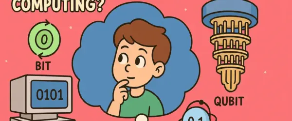
Quantum Computing for Beginners: A Simple Guide
Quantum computing sounds complex and intimidating, but it's simply a new way of solving problems using quantum mechanics principles. You…
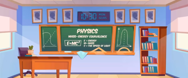
Physics is one of the disciplines of natural sciences which deals with the study of the basic laws of nature and their manifestation in various natural phenomena.
Physicists attempt to explain several diverse natural phenomena in terms of certain scientific laws and concepts.
Quantum computing sounds complex and intimidating, but it's simply a new way of solving problems using quantum mechanics principles. You…
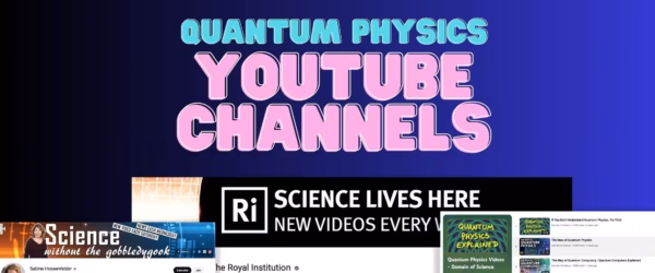
Quantum physics is fascinating and mind-bending, and YouTube channels have made it more accessible than ever. The best quantum physics…

Physics YouTube channels turn one of the most challenging subjects into something genuinely fascinating. The best channels combine rigorous accuracy…

Choosing the right physics textbook can make or break your college experience with the subject. I was a physics major…
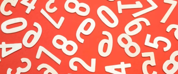
Significant figures seem straightforward until you're in the middle of a multi-step physics or chemistry calculation and realize you've been…
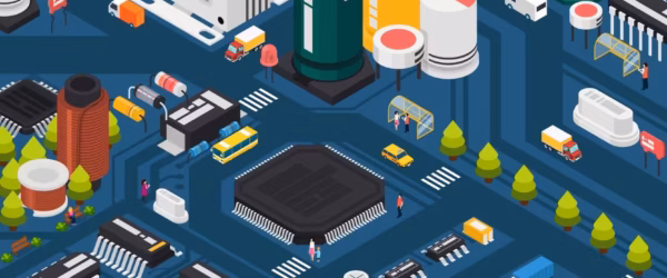
A transistor is a 3-terminal semiconductor switch invented at Bell Labs in 1947. This guide covers what transistors are, how…
Statistical mechanics bridges the gap between microscopic particle behavior and macroscopic thermodynamic properties. Finding the right textbook is crucial because…

General relativity is beautiful, difficult, and absolutely worth learning. Finding the right textbook makes the difference between understanding Einstein's theory…
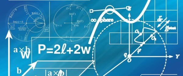
Kinematic equations are the backbone of classical mechanics. If you can't solve projectile motion, free-fall, and acceleration problems confidently, physics…
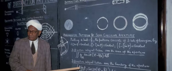
This complete guide covers everything about the Raman Effect. You'll learn about CV Raman's life, the theory behind Raman Scattering,…
Symmetry in physics isn't just about visual balance. It means an operation leaves physical laws unchanged. I explain the deep…
The difference between macrostates and microstates confused me for months in statistical physics. Then a concrete example made everything click.…